Some engineering applications of newly constructed algorithms for one-dimensional non-linear equations and their fractal behavior

1 Introduction

Finding roots of one-dimensional non-linear equations having form $$f(s)=0,$$ where f is a real valued function whose domain is an open connected set, has many applications in applied sciences such as Mathematics, Physics, Engineering etc.

To solve such problems, we have to adopt iterative methods because there does not exist analytical methods that help us to find solutions of such type of problems. In an iteration process, we always need an initial guess, which is improved by processing each iteration. The choice of the initial guess is much important because the speed and performance of the considered algorithm is directly associated with that choice. Some of the classical and basic iterative methods are given in Chen et al. (1993), Burden and Faires (1997), Householder (1970), Kincaid and Cheney (1990), Ostrowski (1966), Traub (1964) and the references are therein.

In the history of polynomials root-finding algorithms, the most widely used algorithm was suggested by Newton in the 17th century, having the following iterative form:

which has quadratic order of convergence.

In recent years, many mathematicians worked on numerical methods using several mathematical techniques for the sake of improving order of convergence and suggested a large number of root-finding algorithms. Some of them are given in He (1999), He (1999), Kumar et al. (2021), Kumar et al. (2021), Kou (2007), Naseem et al. (2021), Naseem et al. (2020), Shah et al. (2016)) and the references are therein.

In twentieth century, Ostrowski (1966) suggested a two-step fourth-order iteration scheme by considering the Newton's method as a predictor. After the work of Ostrowski, Traub (1964) introduced a new fourth-order root-finding algorithm in which he considered the Newton's algorithm as both the predictor and corrector steps. In 2007, Noor et al. (2007) constructed the novel two-step second derivative free Halley's iteration method using the finite difference scheme which possessed the convergence of order five. In 2018, Kumar et al. (2018) introduced a new class of sixth-order parameter-based algorithms for computing zeros of one-dimensional nonlinear equations. In 2020, Behl and Martínez (2020), developed some novel high-order iteration schemes for determining the approximate zeros of non-linear models with convergence orders up to six. These proposed iteration schemes were actually the multidimensional case of the Kou’s method (Kou et al., 2007).

In this paper, we constructed some new iteration schemes which were totally based on the technique of variational iteration. The idea of this technique was first given in 1999 by He (1999). By implementing the described technique, Shah et al. (2016), established some new numerical algorithms to achieve the approximate solution of non-linear scalar equations. The main objective of introducing this thought-provoking idea was to resolve the complex problems associated with non-linear equations (He, 1999a, 1999b; Kou, 2007). The above described technique has been applied to construct higher-order iteration schemes. The suggested schemes are free from higher order derivatives, possessing convergence of sixth-order that becomes the reason of uplifting their efficiency-indices and robust performance. The convergence analysis of the proposed iteration schemes is also given. Several numerical test-examples along with some engineering problems have been included and solved through the proposed schemes which show the better performance and efficiency of the proposed iteration schemes in comparison with the other similar-existing iteration schemes. Using the proposed algorithms, we have generated polynomiographs and compared with other two-step methods of the same kind which represents the fractal behavior of the proposed iteration schemes.

The rest of the paper is organized as follows. The novel iteration schemes are constructed in Section 2. In 3rd Section, the convergence analysis of the suggested schemes is given. In 4th Section, several numerical test-examples including some real-life problems have been solved to demonstrate the validity, applicability, and the performance of the suggested schemes. The graphical representation of the suggested iteration schemes is presented for different complex polynomials in 5th Section which reflects the fractal and dynamic behavior of the suggested iteration schemes. Finally, in the 6th Section, the conclusion of the paper is given.

2 Construction of numerical algorithms using variational iteration technique

This section includes the construction of some new root-finding numerical algorithms for non-linear scalar functions. By means of variational iteration technique, we derived an iteration scheme that involved the auxiliary functions $g$ and by examining a few particular cases of $g$ , we shall deduce some new numerical algorithms. These algorithms are actually two-step iteration schemes, one of which is predictor and other one is known as corrector. These algorithms possess better rate of convergence as compared to single-step methods.

Consider the non-linear algebraic equation:

Assuming “ $\alpha$ ” as a simple zero and “ $\gamma$ ” as the initially chosen guess that is approximately close to “ $\alpha$ ”. Let us denote “ $g(s)$ ” as an arbitrary function and “ $\lambda$ ” to be supposed as a parameter that is called the “Lagrange’s Multiplier” and can be found easily by implementing the optimality-condition. For this purpose, consider the auxiliary function:

By implementing the optimality criteria, the value of $\lambda$ can be found from (3) as:

From (3) and (4):

We apply (5) to obtain the general iteration scheme for deducing numerical algorithms. For this purpose, assume that: $$\mu \left(s\right)=t=s-\frac{f\left(s\right)}{f^{\prime }\left(s\right)}-\frac{f^2\left(s\right)f^{″}\left(s\right)}{2[f^{\prime 3}\left(s\right)-f\left(s\right)f^{\prime }\left(s\right)f^{″}\left(s\right)]},$$

which is cubically convergent, well-known Golbabai-Javidi’s method (Golbabai and Javidi, 2007).

In the light of (4) and (5), one may write:

If $\alpha$ is the root of $f(s)$ , then for $s=\alpha$ , we can write:

Also,

With the help of (7) and (8)

Using (9) in (6), we obtain

which allows us to write the iterative scheme as follows:

where $t_i=s_i-\frac{f\left(s_i\right)}{f^{\prime }\left(s_i\right)}-\frac{f^2\left(s_i\right)f^{″}\left(s_i\right)}{2[f^{\prime 3}\left(s_i\right)-f\left(s_i\right)f^{\prime }\left(s_i\right)f^{″}\left(s_i\right)]}$ .

Relation (11) is the general iteration scheme by means of which, we can derive some novel root-finding numerical algorithms by taking into consideration some specific values of $"g".$

Case-1

Let $g(s_i)=\mathit{exp}(\kappa s_i),$ then $g^{\text{'}}\left(s_i\right)=\kappa g(s_i).$

Putting the above values in (11), gives us an algorithm as defined below:

Case-2

Let $g\left(s_i\right)=exp\left(\kappa f\left(s_i\right)\right),$ then $g^{\prime }\left(s_i\right)=\kappa f^{\prime }\left(s_i\right)g\left(s_i\right).$

Putting the above values in (11), gives us an algorithm as defined below:

Case-3

Let $g\left(s_i\right)=exp\left(-\frac{\kappa }{f\left(s_i\right)}\right),$ then $g^{\prime }\left(s_i\right)=\frac{\kappa f^{\prime }\left(s_i\right)}{f^2\left(s_i\right)}g\left(s_i\right).$

Putting the above values in (11), gives us an algorithm as defined below:

For getting better results for the above described algorithms, always adopt those values of $\kappa$ which maximizes the magnitude of the denominator and prevents it from becoming zero.

3 Convergence analysis

This section includes the convergence analysis of iteration scheme given in (11).

With the help of (12), (13) and (14), we get:

Using equations (12)–(19) in (11), we get $$s_{i+1}=\alpha +\frac{{\left(-c_3+c_2^2\right)}^2[c_{2}g\left(\alpha \right)+g^{\prime }\left(\alpha \right)]}{g\left(\alpha \right)}{e}_i^6+O\left(e_i^7\right),$$

which implies $$e_{i+1}=\frac{{\left(-c_3+c_2^2\right)}^2[c_{2}g\left(\alpha \right)+g^{\prime }\left(\alpha \right)]}{g\left(\alpha \right)}{e}_i^6+O\left(e_i^7\right)$$

The above equality proves that the iteration scheme (11) possesses sixth-order convergence and all the deduced iteration schemes from (11) will possess the same convergence order.

4 Numerical examples

In this part of the paper, we reveal the validity and performance of the proposed iteration schemes by involving three non-linear problems of real life in Engineering and five arbitrary examples which involve non-linear algebraic and transcendental equations. We give a detailed comparison of the suggested schemes with Noor’s iteration method (NR) (Noor et al., 2012), Ostrowski's iteration method (OM) (Ostrowski, 1966) and Traub's iteration method (TM) (Traub, 1964).

We choose the accuracy $\epsilon ={10}^{-15}$ for the stopping-criteria | $s_{i+1}-s_i$ |< $\epsilon$ . We use the computer program Maple-13 for solving the numerical test-examples.

Example 4.1. Fractional Conversion

We consider this example from Balaji and Seader (1995), that explains the fractional conversion of nitrogen–hydrogen feed to ammonia. By taking the values of the pressure and temperature as 250 atm and ${500}^0$ C respectively, the present problem has been converted to the following form: $$0.186+\frac{8{s^2\left(s-4\right)}^2}{9{\left(s-2\right)}^3}=0$$

which may be converted to the form of non-linear function as:

${f_1\left(s\right)=s}^4-7.79075{\mathrm{s}}^3+14.7445{\mathrm{s}}^2+2.511s-1.674$ .

As the degree of polynomial, given in the above equation is four, so it must possess exactly four roots according to the fundamental theorem of Algebra. Obviously, the fraction conversion has values between (0,1) interval, so there exists only one real-root 0.2777595428 in (0,1) interval. The remaining roots of the above function do not have any physical meaning. We initialize the process of iteration by choosing the starting point as $s_0=0.5$ .

Example 4.2. Finding Volume from Van Der Wall’s Equation

In Chemistry and Chemical Engineering, the van der Waal’s equation is utilized for examining the behavior of real and ideal gases (Waals and Diderik, 1873) and has the following form: $$\left(P+\frac{A_1{n}^2}{V^2}\right)\left(V-n{A}_2\right)=nRT,$$

By adopting the particular values of the parameters in the above given equation, one may convert it easily to the non-linear equation given as: $$f_2\left(s\right)=0.986{\mathrm{s}}^3-5.181{\mathrm{s}}^2+9.067\mathrm{s}-5.289,$$ where $s$ stands for the volume which can be determined by solving the non-linear function $f_2$ . As the above given polynomial has three degree, so it must have exactly three roots and among of them, there exists only one feasible positive real-root 1.9298462428 because the numerical value of the volume cannot be negative for gases. We initialize the iteration process by choosing the starting guess $s_0=3.9$ .

Example 4.3. Fractional-Transformation in a Chemical Reactor Problem

Regarding the fractional-transformation of a particular specie, say M in the chemical reactor problem (Shacham, 1986), the following non-linear equation can be considered: $$f_3\left(s\right)=\frac{s}{1-s}-5\ln \left[\frac{0.4(1-s)}{0.4-0.5s}\right]+4.45977,$$ where the variable $s$ denotes the fractional-transformation of the specie in the reactor. It should be noted that the non-linear expression of the function $f_3$ would be meaningless physically for the negative values of s because outside of the bounded region (0,1) its derivative does not exist, and we are unable to proceed further. Therefore, for the starting of the iteration process, the starting point should be chosen carefully inside the region (0,1) for computing the approximate zero of the function $f_3$ . In this example, we start the iteration process with the initial guess $s_0=0.79$ .

Example 4.4. Algebraic and Transcendental Equations

To numerically analyze the suggested algorithms, we consider the following five algebraic and transcendental equations: $$f_4\left(s\right)=s^3+4s^2-15,f_5\left(s\right)=({s-1)}^3-1,f_6\left(s\right)=\cos \left(s\right)+e^{-s},$$ $$f_7\left(s\right)=s^{10}-1,f_8\left(s\right)=s+\ln \left(s\right).$$

Table 1 gives us the detailed comparison of the suggested iteration schemes with other similar existing iteration schemes numerically. In the columns of the presented table, the symbol $N$ stands for the no. of iterations, $|f(s)|$ stands for the absolute value of $f(s)$ , $s_{i+1}$ stand for the final approximated root and the computational order of convergence (COC) which can be approximated using the following formula: $$\mathit{COC}\approx \frac{\mathit{ln}\frac{|s_{i+1}-\alpha |}{|s_i-\alpha |}}{\mathit{ln}\frac{|s_i-\alpha |}{|s_{i-1}-\alpha |}}$$

The above approximation was first introduced in Weerakoon and Fernando (2000).

Table 2 gives us the comparison of the suggested iteration schemes with the other similar ones in terms of the number of iterations for the higher accuracy $\epsilon ={10}^{-100}$ . In the presented table, the columns display the quantity of iterations taken by the iteration schemes for different non-linear functions with the initial guess $s_0.$ We made all the calculation with the aid of the computer program Maple-13.

5 Graphical representation

The aim of this section is to present a detailed graphical comparison of the proposed iteration schemes with the other similar existing methods in literature through the generated polynomiographs for different complex polynomials. A polynomiograph is a particular image which generates as a result of the process, called polynomiography. This term was first introduced by Kalantari (2005) and defined as “the art and science of visualization in approximation of the zeros of complex polynomials, via fractal and non-fractal images created using the mathematical convergence properties of iteration functions” (Kalantari, 2005). The word “fractal” that is actually a geometrical image, having each part the same statistical character as the entire, was first introduced by the Mandelbrot (1983). The polynomiographs and fractals, both can be achieved through a variety of numerical algorithms. The polynomiographs and fractals are quite different from each other in terms of structure scale. The “polynomiographer” can modulate the structure and pattern systematically by means of different numerical algorithms, applied to a variety of complex polynomials. Generally, the polynomiographs and fractals are members of distinct families of graphical objects.

To generate polynomiographs using computer program through different numerical algorithms, we must choose a starting region in the form of the rectangle $\mathcal{R}$ that contains the zeros of the considered complex polynomial and then corresponding to every point $w_0$ in that region, we execute the process of iteration and coloring the point corresponding to $w_0$ which relies upon the approximate convergence of truncated orbit to a root, or lack thereof. The generated image’s resolution totally relies upon the discretization of the rectangle. For instance, discretization of rectangle into a $2000$ by $2000$ grid results a high-resolution image.

Usually, polynomiographs’ colors are purely associated with the iterations needed to approximate the zeros of the complex polynomial for the given accuracy and the considered algorithm. The most general algorithm for polynomiograph’s generation is presented in Algorithm 4.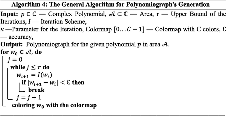

Close

Export to PPT

In a numerical algorithm which involves the iteration process, there is always a need of the stopping criterion for the whole process, i.e., a test that informs us about the convergence or divergence of the considered algorithm. Such a test is usually called the convergence test with the standard form given as:

We consider the following complex polynomials for the generation of polynomiographs through the constructed iteration schemes and compare them with those obtained through the other well-known similar existing iteration schemes. $$p_1\left(w\right)=w^3-1,p_2\left(w\right)={(w^3-1)}^2,p_3\left(w\right)=w^4-1,p_4\left(w\right)={(w^4-1)}^2,p_5\left(w\right)=w^5-1,p_6\left(w\right)={(w^5-1)}^2.$$

The colormap used for the coloring of iterations in the generation of polynomiographs

Fig. A

Close

Fig. A

The colormap used for generating polynomiographs.

Export to PPT

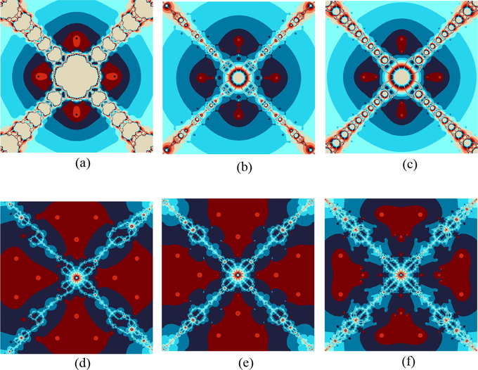
Example 5.1. Polynomiographs for the Polynomial $p_1\left(w\right)$ Using Various Iterative Methods

Close

Fig. 1

Polynomiographs associated with the polynomial $p_1\left(w\right)$ . (a) stands for Noor’s method, (b) stands for Ostrowski’s method, (c) stands for Traub’s method, (d), (e) and (f) stand for Algorithms 1–3 respectively.

Export to PPT

Example 5.2. Polynomiographs for the Polynomial $p_2\left(w\right)$ Using Various Iterative Methods

Close

Fig. 2

Polynomiographs associated with the polynomial $p_2\left(w\right)$ . (a) stands for Noor’s method, (b) stands for Ostrowski’s method, (c) stands for Traub’s method, (d), (e) and (f) stand for Algorithms 1–3 respectively.

Export to PPT

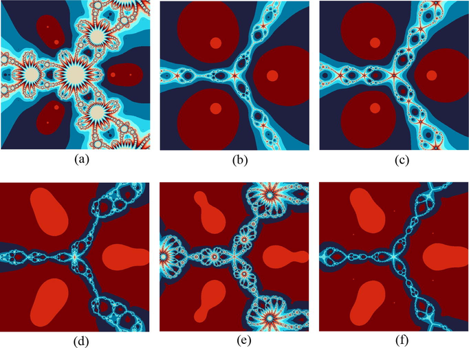
Example 5.3. Polynomiographs for the Polynomial $p_3\left(w\right)$ Using Various Iterative Methods

Close

Fig. 3

Polynomiographs associated with the polynomial $p_3\left(w\right)$ . (a) stands for Noor’s method, (b) stands for Ostrowski’s method, (c) stands for Traub’s method, (d), (e) and (f) stand for Algorithms 1–3 respectively.

Export to PPT

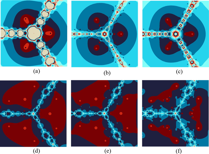
Example 5.4. Polynomiographs for the Polynomial $p_4\left(w\right)$ Using Various Iterative Methods

Close

Fig. 4

Polynomiographs associated with the polynomial $p_4\left(w\right)$ . (a) stands for Noor’s method, (b) stands for Ostrowski’s method, (c) stands for Traub’s method, (d), (e) and (f) stand for Algorithms 1–3 respectively.

Export to PPT

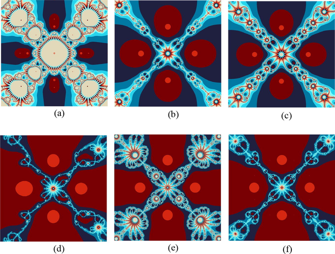
Example 5.5. Polynomiographs for the Polynomial $p_5\left(w\right)$ Using Various Iterative Methods

Close

Fig. 5

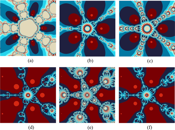
Polynomiographs associated with the polynomial $p_5\left(w\right)$ . (a) stands for Noor’s method, (b) stands for Ostrowski’s method, (c) stands for Traub’s method, (d), (e) and (f) stand for Algorithms 1–3 respectively.

Export to PPT

Example 5.6. Polynomiographs for the Polynomial $p_6\left(w\right)$ Using Various Iterative Methods

Close

Fig. 6

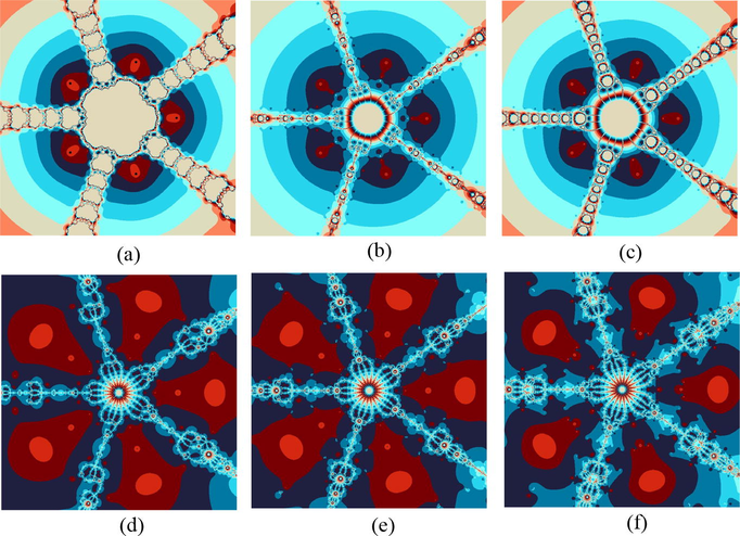
Polynomiographs associated with the polynomial $p_6\left(w\right)$ . (a) stands for Noor’s method, (b) stands for Ostrowski’s method, (c) stands for Traub’s method, (d), (e) and (f) stand for Algorithms 1–3 respectively.

Export to PPT

In examples 5.1–5.6, we compared the dynamics of the suggested algorithms with the other similar ones in the form of polynomiographs for the different complex with the aid of computer technology. In the first example, we executed all the iteration schemes to achieve the zeros of the cubic polynomial $p_1\left(w\right)$ . The results of the polynomiographs are given in Fig. 1. In 2nd example, we executed the iteration schemes for polynomial $p_2\left(w\right)$ that possess three distinct zeros of multiplicity 2. The corresponding polynomiographs are presented in Fig. 2. The repeated roots appeared with the same color and location on the corresponding polynomiographs. In 3rd and 4th examples, we ran the iteration schemes for polynomials $p_3\left(w\right)$ and $p_4\left(w\right)$ . The corresponding results are shown in Figs. 3 and 4. These polynomials possess four distinct zeros and their polynomiographs have been shown in Figs. 3 and 4 respectively. The second polynomial $p_4\left(w\right)$ possesses all the zeros of multiplicity 2. The polynomiographs for $p_5\left(w\right)$ and $p_6\left(w\right)$ through the proposed iteration schemes have shown in Figs. 5 and 6 respectively. These two polynomials possess five distinct zeros but the zeros of the second one i.e., $p_6\left(w\right)$ are not simple and of multiplicity 2 and can be seen easily on the complex plane of the corresponding polynomiographs.

By studying these graphical objects keenly, one can analyze two major features of the considered iteration schemes. One of them is the convergence speed or rate of the iteration scheme, i.e., the coloring of each point informs us about the quantity of iterations that were consumed by the iteration scheme for finding the approximate root. The 2nd feature is the dynamics of the considered iteration scheme. The regions of the plane where the variation of colors is minimum, the dynamics would be low, whereas in the regions with large variation of colors, the dynamics must be higher. The black color points out that regions of the plane in which there is no possibility to attain the required solution of the given problem for the given number of iterations. The appearance of darker region in the above presented images shows that the considered algorithm requires less number of iterations. The same-color regions that appeared in above presented figures showing the similar consumption of iterations to attain the required solution and they look alike to the contour lines on the map. It can be noted that the polynomiographs generated through our developed algorithms contained much brighter and darker areas and did not contain black area as compared to other two-step algorithms of same kind which showing the superiority of the proposed algorithms over the other ones. Also, the polynomiographs of the suggested algorithms showing the larger convergence area than the other comparable methods which proves the better efficiency of the suggested algorithms.

We generated all the graphical objects with the aid of computer program Mathematica $12.0$ for $\epsilon =0.001$ and $r=15$ where the symbol $\epsilon$ stands for the accuracy and $r$ denotes the upper bound of the number of iterations.

6 Conclusion

Based upon the main idea of variational iteration technique, we established some novel sixth-order iteration schemes for finding roots of the one-dimensional non-linear equations. By including some numerical test-examples, the validity, applicability and performance of the suggested iteration schemes are also discussed. These examples also include some real-life application associated with the chemical engineering. The numerical results of these test-examples uphold the analysis of the convergence that is shown in Tabs. 1–2. The suggested iteration schemes showing better results in respect of efficiency, consumption of iterations, and the computational order of convergence against the other well-known similar nature two-step iteration schemes. The dynamics of the suggested iteration schemes in the form of the polynomiographs of different complex polynomials have been analyzed. The presented graphical images look esthetically pleasing, richer, colorful and have very interesting and complex patterns that revealed the fractal behavior and other dynamical aspects of the suggested iteration schemes.

7 Author’s contributions

All authors contributed equally to the writing of this paper. All authors read and approved the final manuscript.

References

- Application of interval Newton’s method to chemical engineering problems. Reliab. Comput.. 1995;1(3):215-223.
- [Google Scholar]
- A new high-order and efficient family of iterative techniques for nonlinear models. Complexity. 2020;2020:1-11.
- Numerical Analysis (6th ed.). California, USA: Brooks/Cole Publishing Company; 1997.
- A note on the Halley method in Banach spaces. Appl. Math. Comput.. 1993;58(2-3):215-224.
- Fractal patterns from the dynamics of combined polynomial root finding methods. Nonlinear Dyn.. 2017;90(4):2457-2479.
- Visual analysis of the Newton’s method with fractional order derivatives. Symmetry. 2019;11(9):1143.
- [CrossRef] [Google Scholar]
- A third-order Newton type method for nonlinear equations based on modified homotopy perturbation method. Appl. Math. Comput.. 2007;191(1):199-205.
- Variational iteration method–a kind of nonlinear analytical technique: Some examples. Int. J. Non Linear Mech.. 1999;34(4):699-708.
- Homotpy perturbation technique. Comput. Methods Appl. Mech. Eng.. 1999;178:257-262.
- The Numerical Treatment of a Single Nonlinear Equation. New York: USA, McGraw-Hill; 1970.
- Polynomiography from the fundamental theorem of Algebra to art. Leonardo. 2005;38(3):233-238.
- Kalantari, B., 2005. Method of creating graphical works based on polynomials. U.S. Patent 6, 894, 705.
- Polynomiography via modified Abbasbanday's method. Int. J. Math. Anal.. 2017;11:133-149.
- Numerical Analysis. Pacific Grove, California, USA,: rooks/Cole Publishing Company; 1990.
- The improvements of modified Newton's method. Appl. Math. Comput.. 2007;189(1):602-609.
- A composite fourth-order iterative method for solving non-linear equations. Appl. Math. Comput.. 2007;184(2):471-475.
- Lie symmetry analysis for obtaining the abundant exact solutions, optimal system and dynamics of solitons for a higher-dimensional Fokas equation. Chaos, Solitons Fractals. 2021;142:110507.
- Lie symmetries, optimal system and group-invariant solutions of the (3+1)-dimensional generalized KP equation. Chinese J. Phys.. 2021;69:1-23.
- A family of higher order iterations free from second derivative for nonlinear equations in R. J. Comput. Appl. Math.. 2018;330:215-224.
- The Fractal Geometry of Nature, New York, USA. W. H. Freeman and Company; 1983.
- Higher-order root-finding algorithms and their basins of attraction. J. Math.. 2020;2020:1-11.
- Numerical algorithms for finding zeros of nonlinear equations and their dynamical aspects. J. Math.. 2020;2020:1-11.
- Some new iterative algorithms for solving one-dimensional non-linear equations and their graphical representation. IEEE Access. 2021;9:8615-8624.
- Basins of attraction for several methods to find simple roots of nonlinear equations. Appl. Math. Comput.. 2012;218(21):10548-10556.
- A new modified Halley method without second derivatives for nonlinear equation. Appl. Math. Comput.. 2007;189(2):1268-1273.
- Some new iterative methods for solving nonlinear equations. World Appl. Sci. J.. 2012;20:870-874.
- Solution of Equations and Systems of Equations (second ed.). Academic Press; 1966.
- Numerical solution of constrained non-linear algebraic equations. Int. J. Numer. Meth. Eng.. 1986;23(8):1455-1481.
- Some second-derivative-free sixth-order convergent iterative methods for non-linear equations. Maejo Int. J. Sci. Technol.. 2016;10:79-87.
- A new family of optimal eighth order methods with dynamics for non-linear equations. Appl. Math. Comput.. 2016;273:924-933.
- Iterative Methods for Solution of Equations. Englewood, Cliffs, NJ: Prentice-Hall; 1964.
- Waals, V. D., Diderik, J., 1873. Over de continuiteit van den gas-en vloeistoftoestand (on the continuity of the gas and liquid state). Ph.D. dissertation, Leiden, The Netherlands.
- A variant of Newton’s method with accelerated third-order convergence. Appl. Math. Lett.. 2000;13(8):87-93.