

Solution of fractional-order differential equations based on the operational matrices of new fractional Bernstein functions
⁎Corresponding author. alshbool.mohammed@gmail.com (M.H.T. Alshbool)
-
Received: ,
Accepted: ,
This article was originally published by Elsevier and was migrated to Scientific Scholar after the change of Publisher.
Peer review under responsibility of King Saud University.
Abstract
An algorithm for approximating solutions to fractional differential equations (FDEs) in a modified new Bernstein polynomial basis is introduced. Writing
Keywords
Bernstein polynomials
Fractional differential equation
Error analysis

1 Introduction
Fractional differential equations have several applications in mathematical physics, fluid flow, engineering and other areas of applications (Miller and Ross, 1993; Podlubny, 1999; Jafari and Momani, 2007; Daftardar and Jafari, 2007; Abdulaziz et al., 2008). In this paper, we consider the fractional differential equations (FDEs) of the form:
Numerical and analytical methods are applied to solve fractional differential equation such as homotopy perturbation method (Hosseinnia et al., 2008), Modification of homotopy perturbation methods (Odibat and Momani, 2008), Taylor collocation method (Cenesiz et al., 2010), Jacobi operational matrix method (Kazem, 2013), Variational iteration method (Odibat and Momani, 2006), Legendre functions method (Kazem et al., 2013), Tau methods (Rad et al., 2014), A new operational matrix method (Saadatmandi and Dehghan, 2010). Yang et al. (2015) presented local fractional derivative operators and local integral transforms to solve fractional differential equations. Rostamya et al. (2013) proposed anew efficient basis to solve fractional partial differential equations.
Fractional Riccati differential equations have been solved by many efficient techniques such as Adomian’s decomposition method (Gejji and Jafari, 2007; Momani and Shawagfeh, 2006) and new spectral wavelets methods (Abd-Elhameed and Youssri, 2014).
One of the most important numerical methods for solving linear and nonlinear equations is Bernstein polynomials which have been used by many authors. Pandey and Kumar (2012) used Bernstein operational matrix of differentiation to solve Lane–Emden type equation. Besides that Bhatti and Bracken (2007) solved the differential equations by using Galerkin method based on the Bernstein polynomial basis. Yousefi and Behroozifar (2010) presented an operational matrix method based on Bernstein polynomials for the differential equations. Recently, Yiming et al. (2014) solved a variable order time fractional diffusion equation using Bernstein polynomials. Alshbool and Hashim (2016) presented multistage Bernstein polynomials which is a new modification of Bernstein polynomials to find the solutions of fractional order stiff systems.
In the present paper, we utilize a new operational matrices method based on the Bernstein polynomials to solve linear and non-linear fractional differential equations. We generalize r for
This article is structured as follows. In Section 2, the definitions and properties of the fractional calculus are given. In Section 3, our method and its applications are explained. In Section 4, an error analysis of the method and estimation of the error are presented, as well as the corrected absolute error. In Section 5, our numerical findings, exact solution and demonstration of the validity, accuracy and applicability of the operational matrices by considering numerical examples are reported. Section 6, consists of brief summary and conclusion.
2 Preliminaries and notations
In this section, we provide some definitions and properties of the fractional calculus (Diethelm et al., 2005; Podlubny, 1999).
A real function
The Riemann–Liouville fractional integral operator
-
-
-
The fractional derivative
The following are two basic properties of the Caputo fractional derivative (Miller and Ross, 1993):
-
Let
-
Let
For the Caputo derivative we have
3 Description of the method
To solve (1), (2) by developing the Bernstein polynomial approximation with the help of the matrix operations, the collocation method and the caputo fractional derivative are used. We obtain an approximate solution of the problem (1), (2) in the form of
Substituting (
Firstly, Eq. (10) is applied to approximate
4 Error analysis and estimation of the absolute error
In this section,we present the error analysis of the method used. Residual correction procedure which may estimate the absolute error will be assigned for the problem.
Let
First, adding and subtracting the term
Let
We term the approximate solution
5 Illustrative examples
To illustrate the effectiveness of the presented method, the following examples of linear and non-linear fractional differential equations (FDEs) are provided.
Consider the fractional differential equation which has been considered by Saadatmandi and Dehghan (2010).
Consider the nonlinear fractional differential equation which has been considered by Yüzbası (2013).
Consider the nonlinear fractional differential equation which has been considered by Yüzbası (2013).
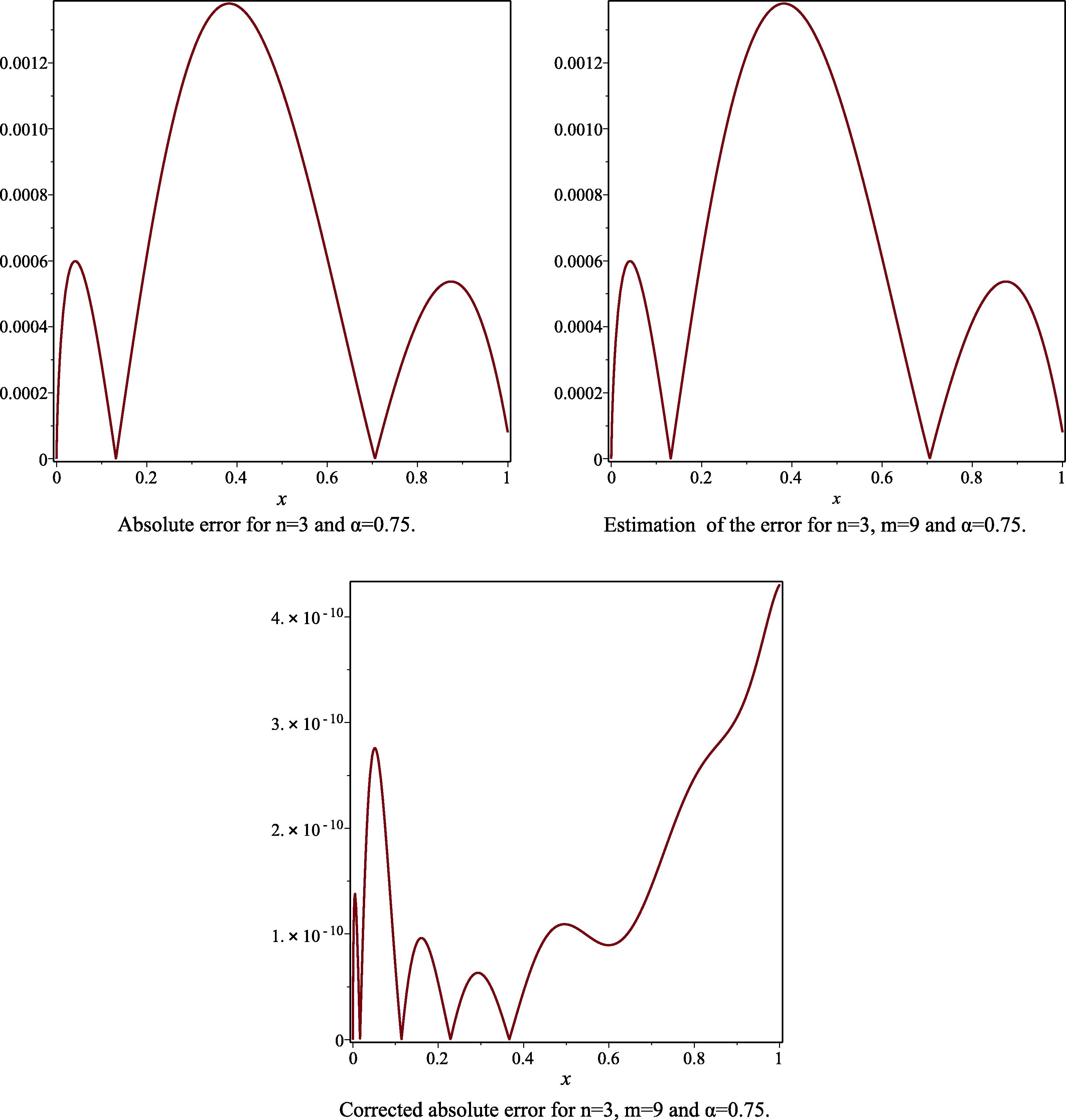
- The absolute error, the estimated absolute error and the corrected absolute error to Example 1, for the case
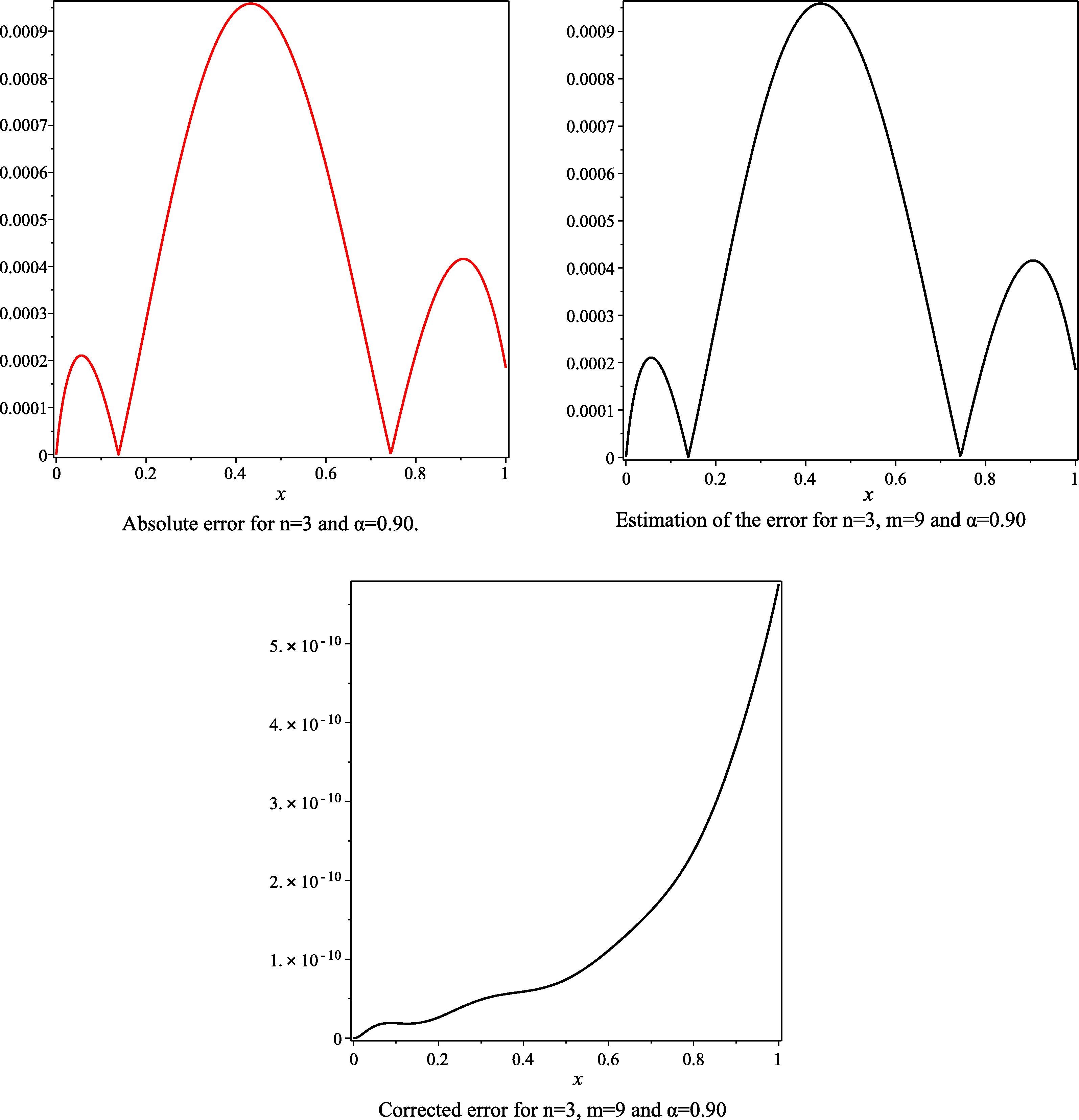
- The absolute error, the estimated absolute error and the corrected absolute error to Example 1, for the case
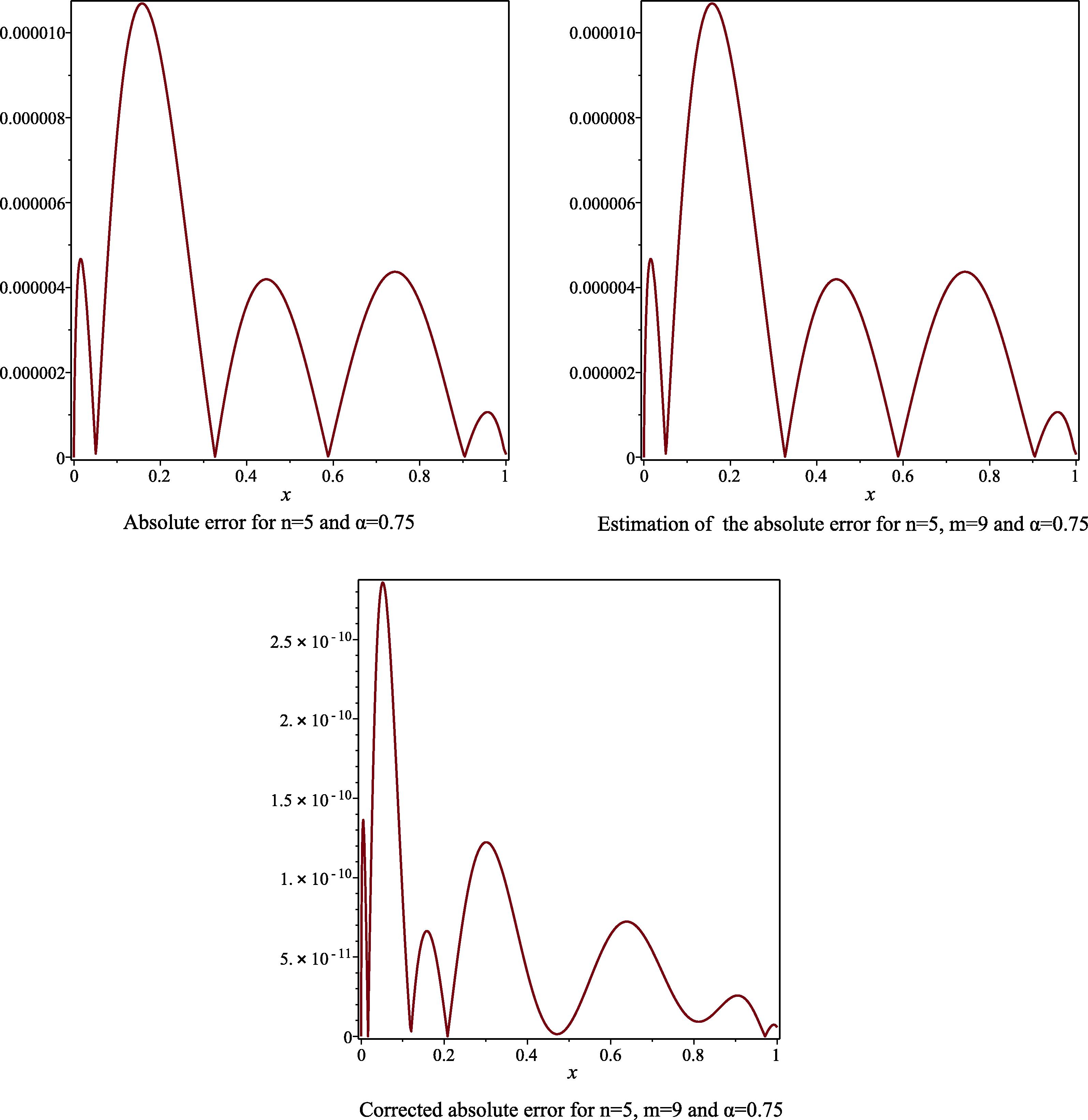
- The absolute error, the estimated absolute error and the corrected absolute error to Example 1, for the case
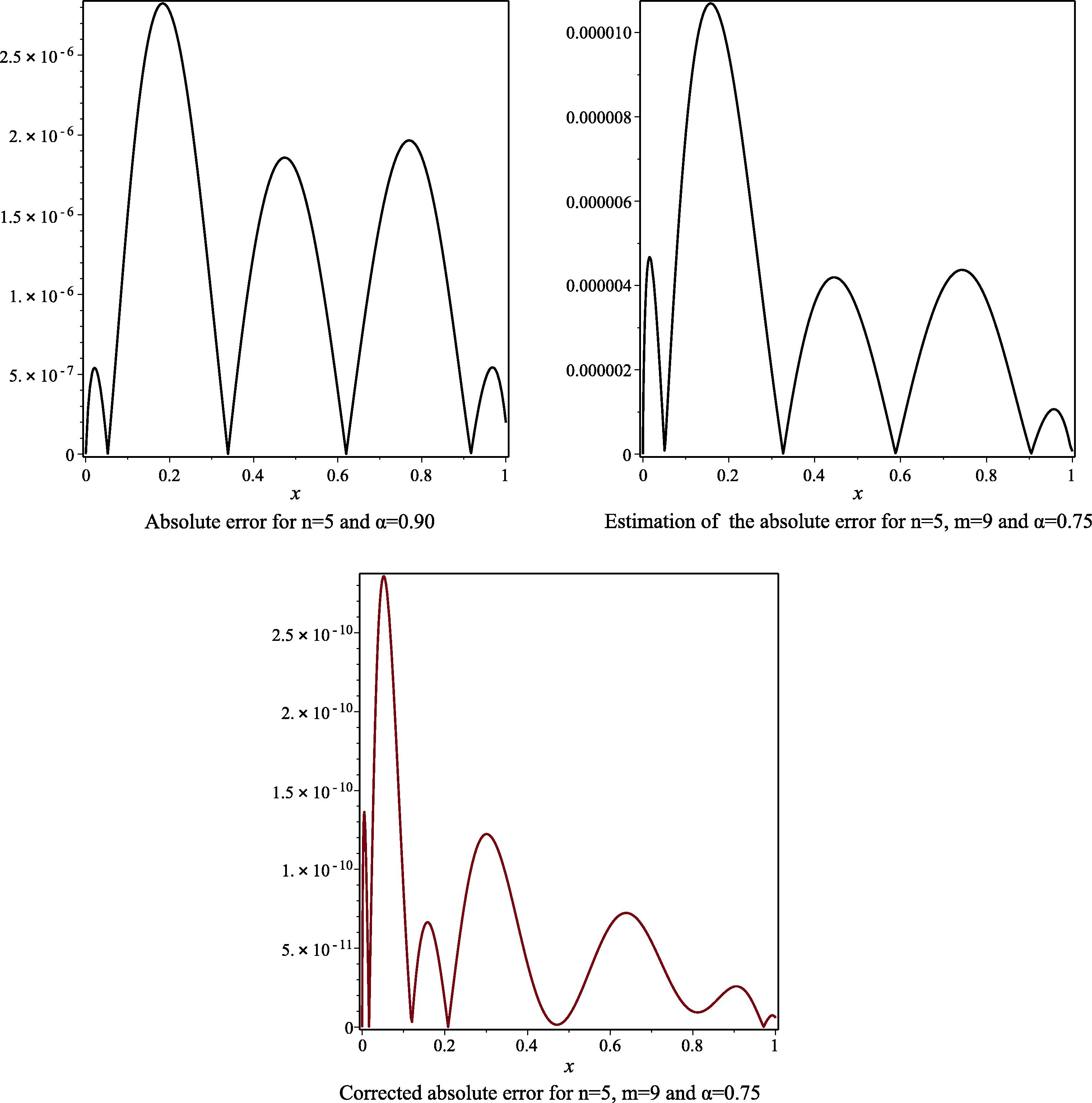
- The absolute error, the estimated absolute error and the corrected absolute error to Example 1, for the case
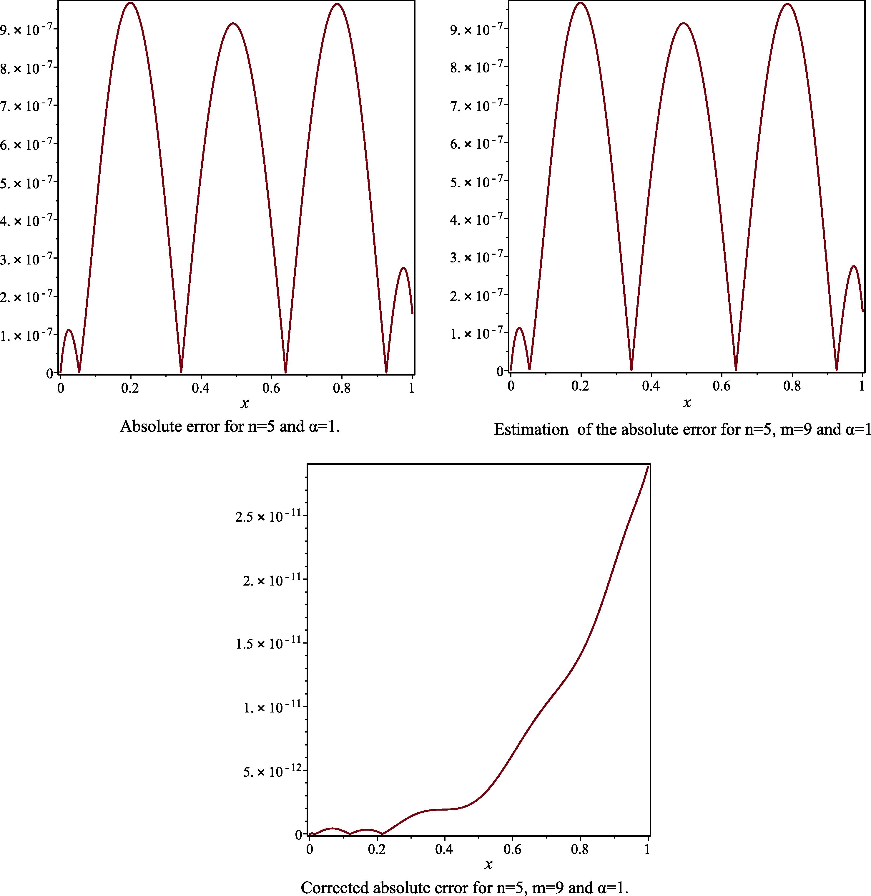
- The absolute error, the estimated absolute error and the corrected absolute error to Example 1, for the case
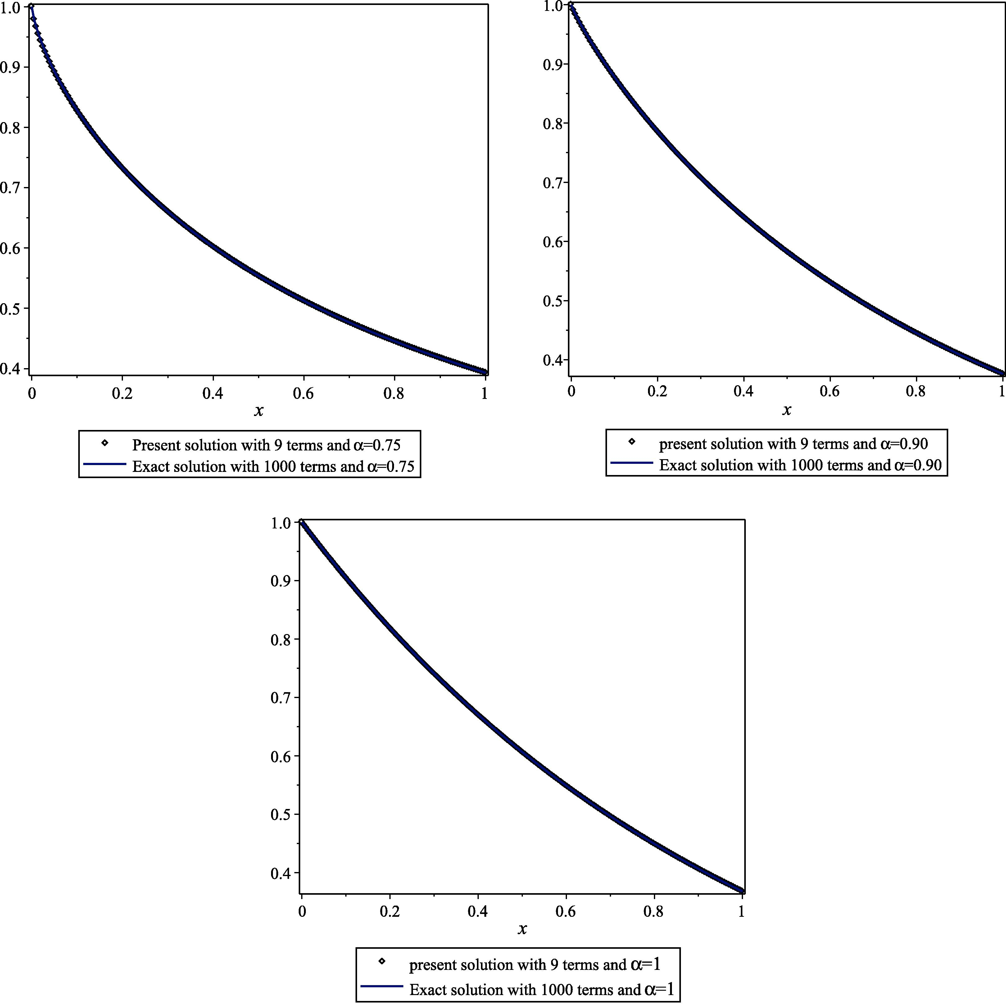
- Compare between our present solution with terms 9 and Exact solution with 1000 terms.
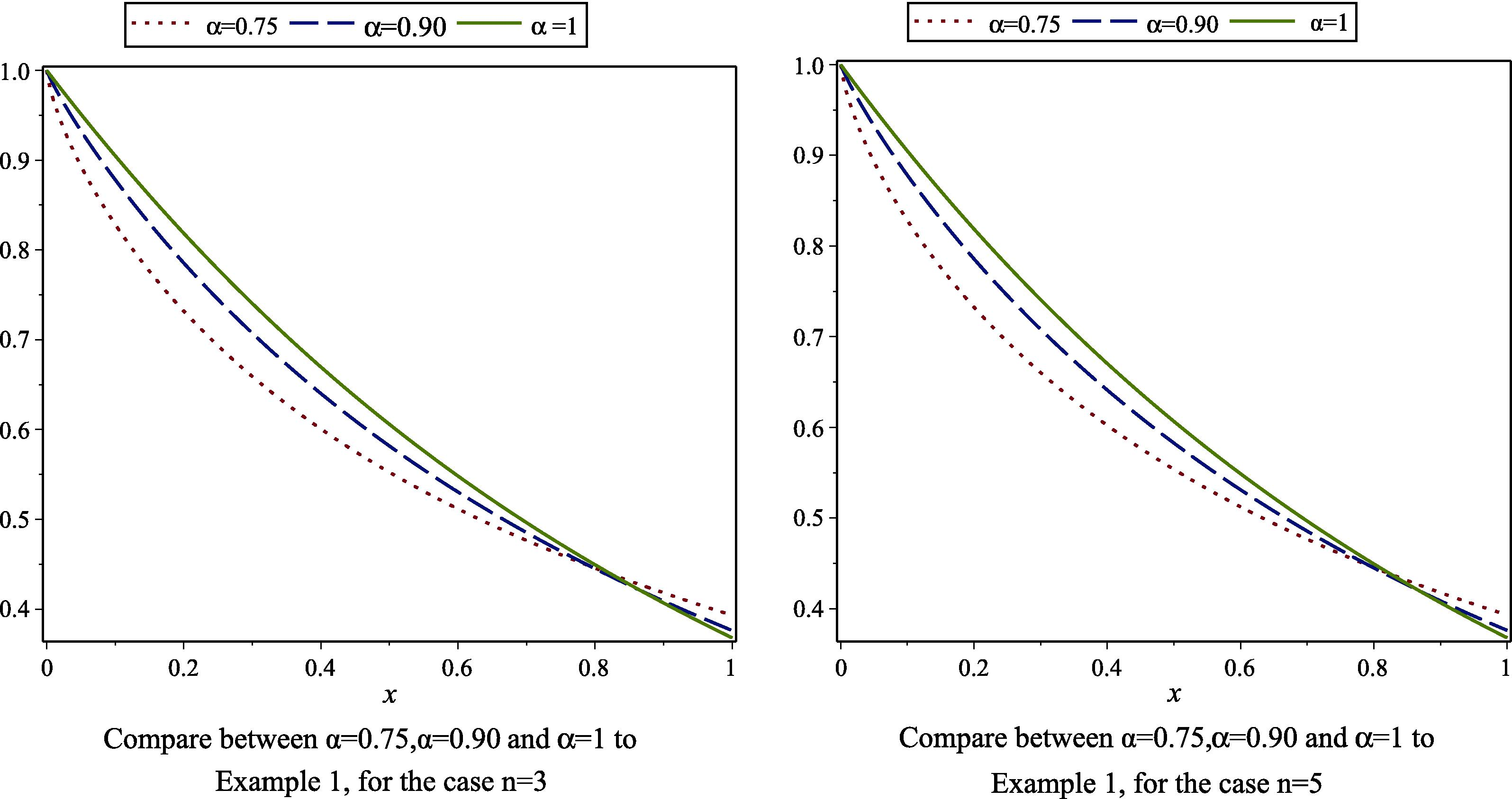
- Compare between
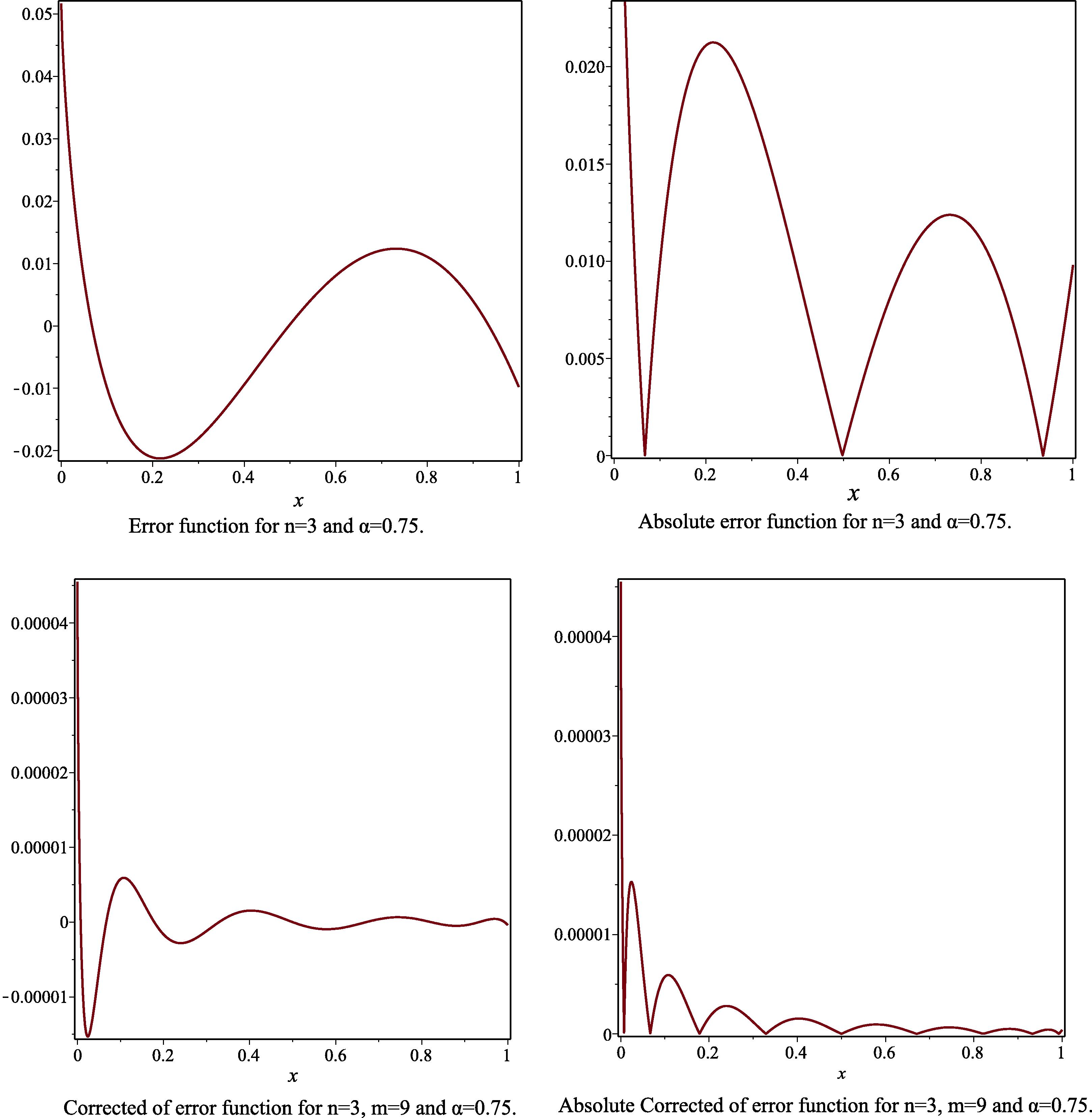
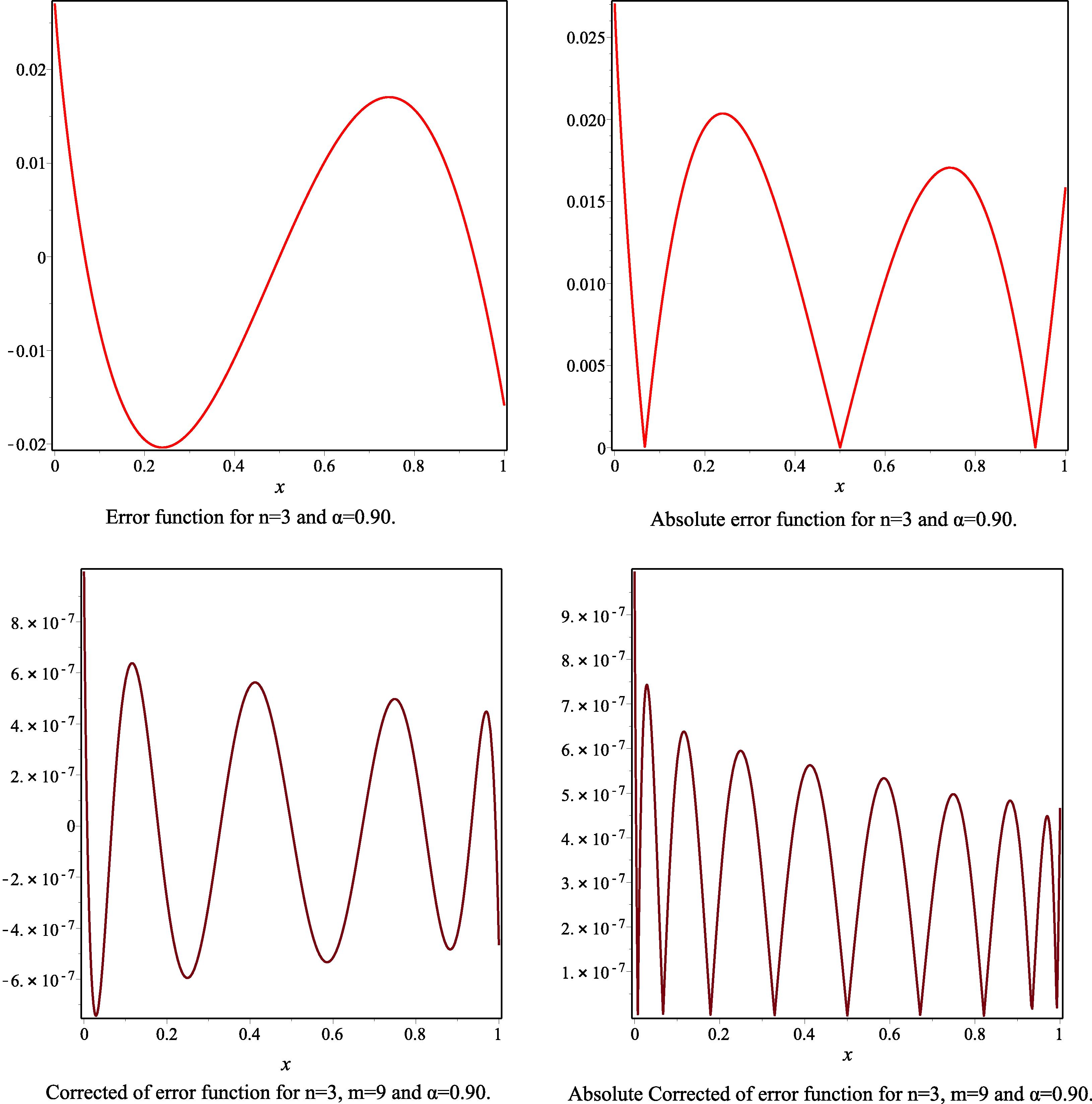
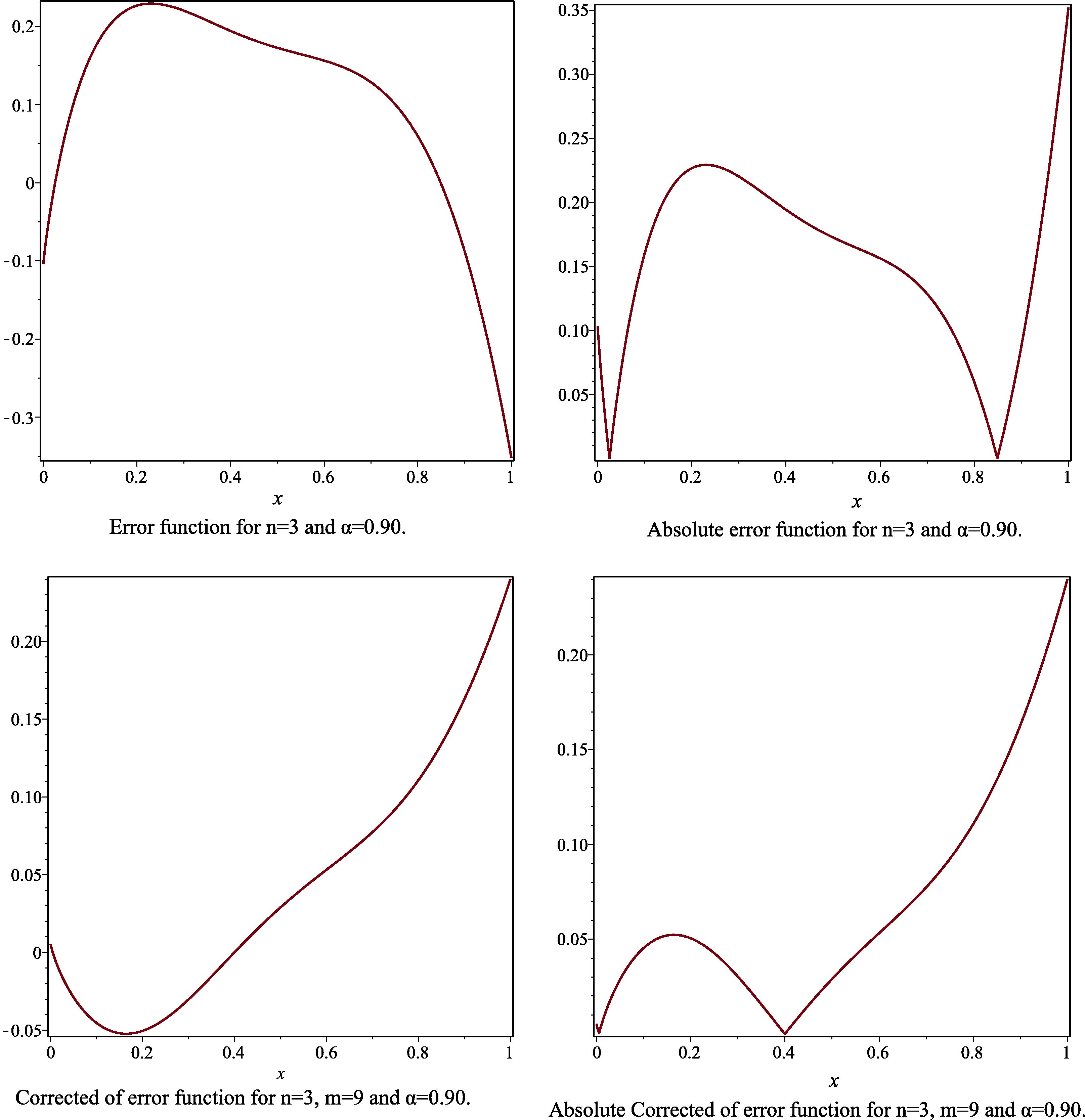
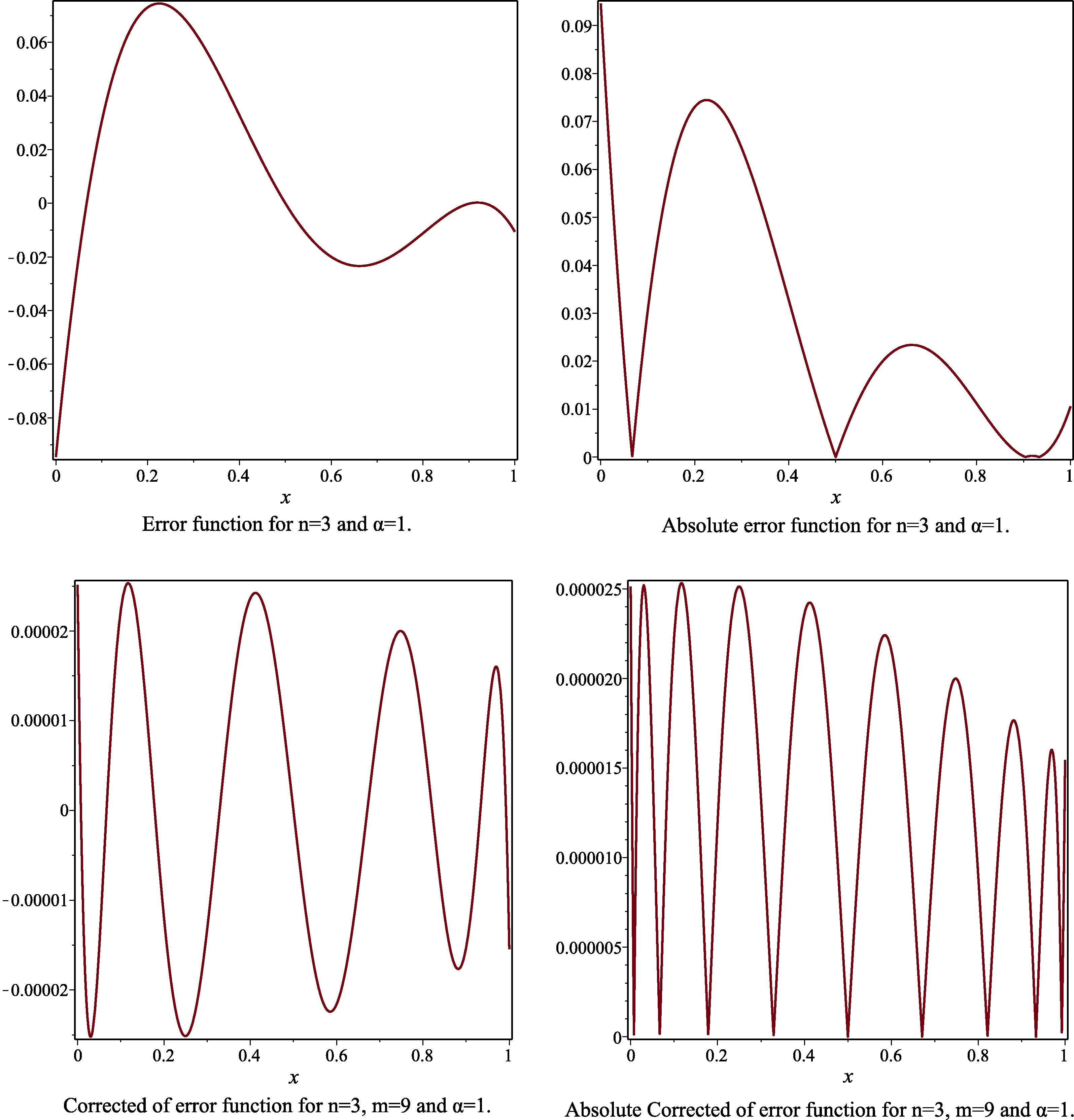
- The error function, the absolute of error function, the corrected error function and the absolute corrected error function to Example 2, for the case
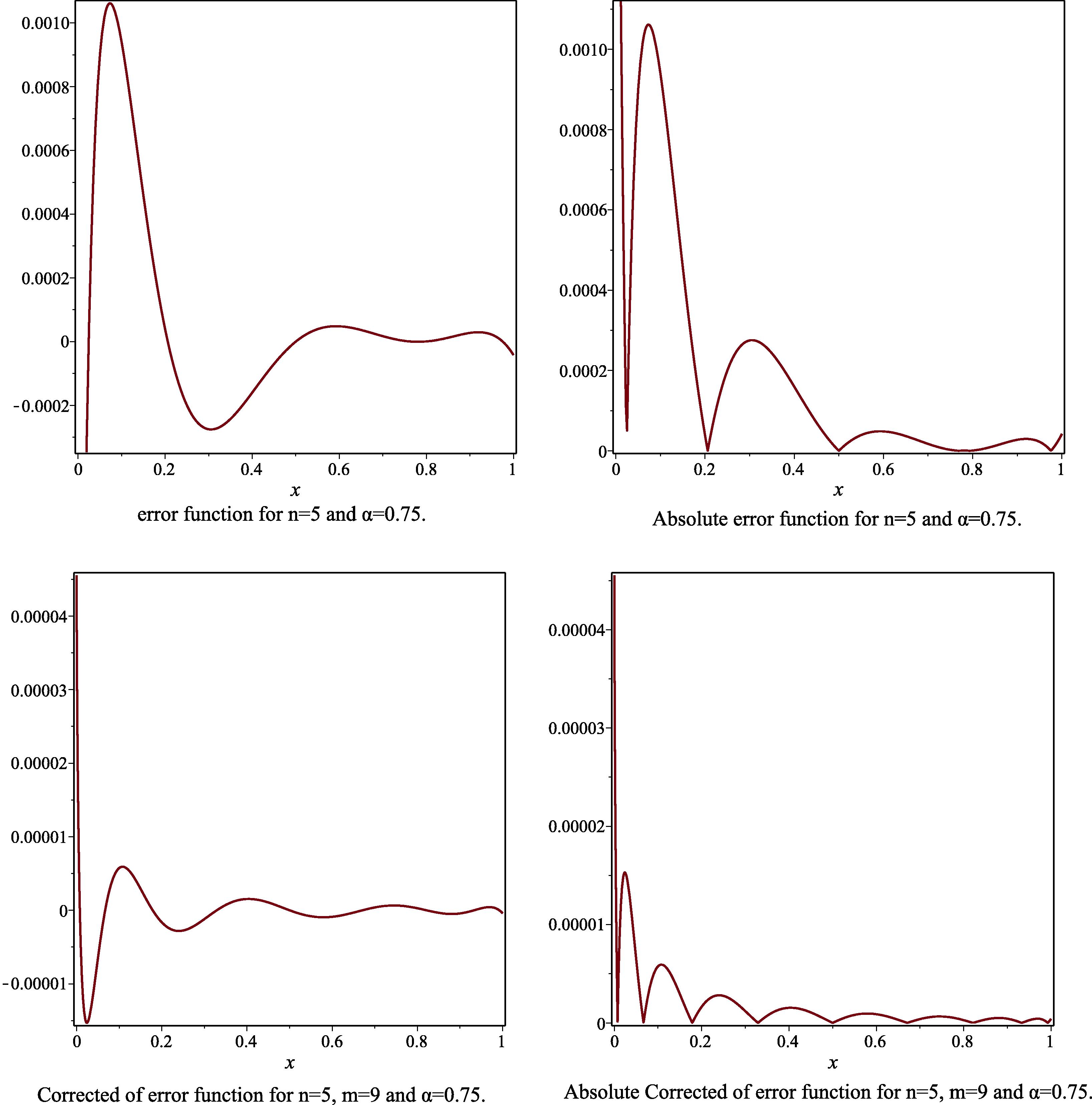
- The error function, the absolute of error function, the corrected error function and the absolute corrected error function to Example 2, for the case
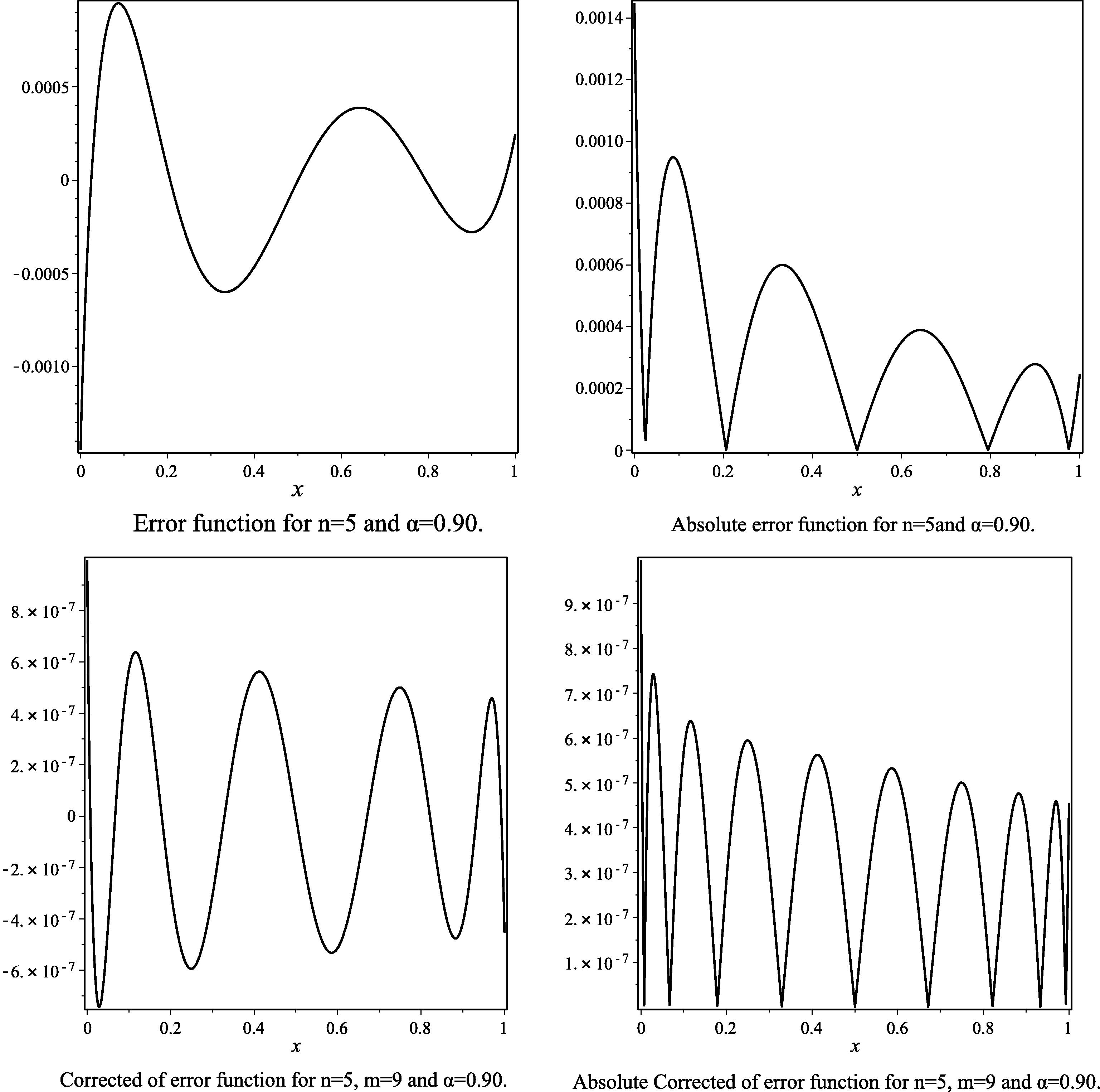
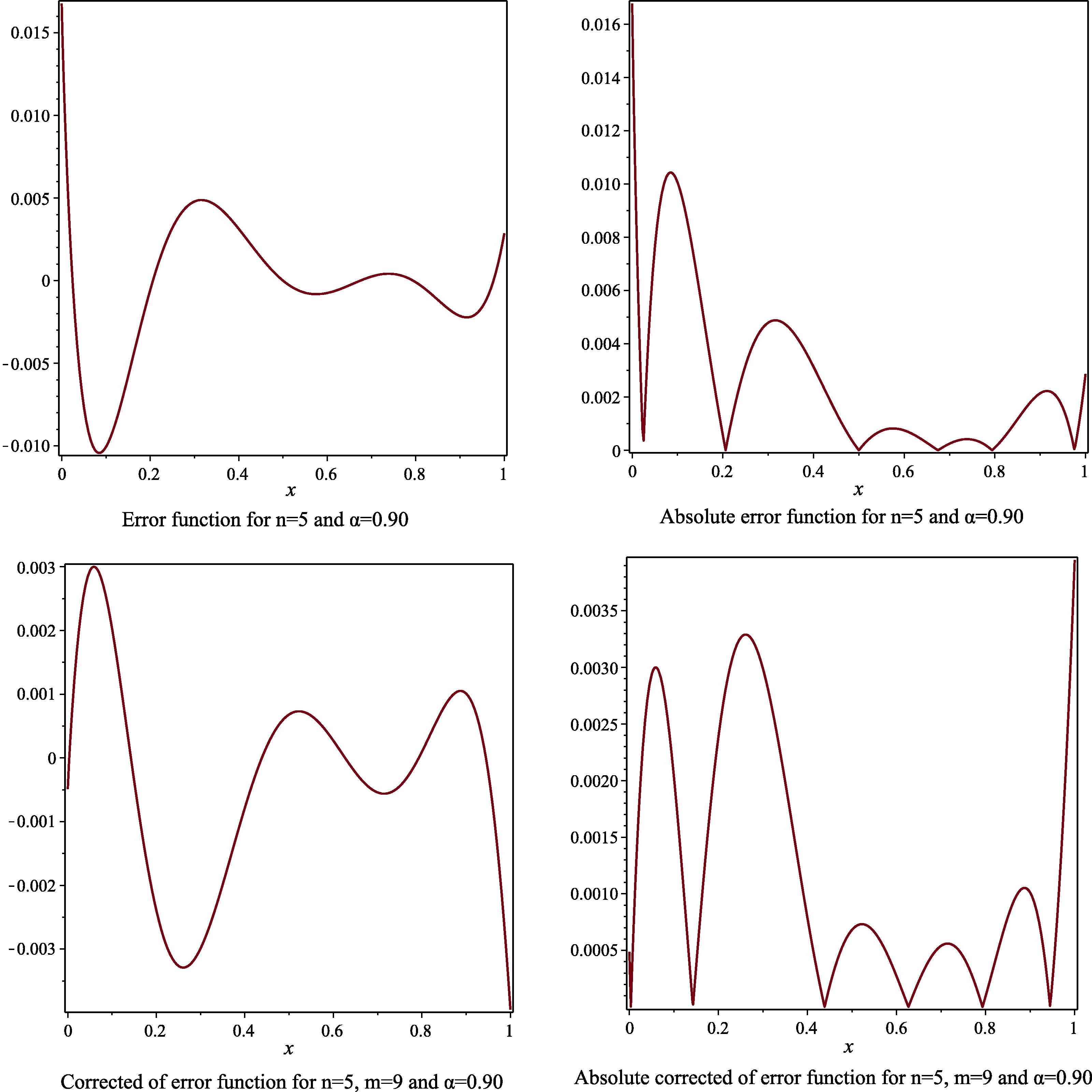
- The error function, the absolute of error function, the corrected error function and the absolute corrected error function to Example 2, for the case
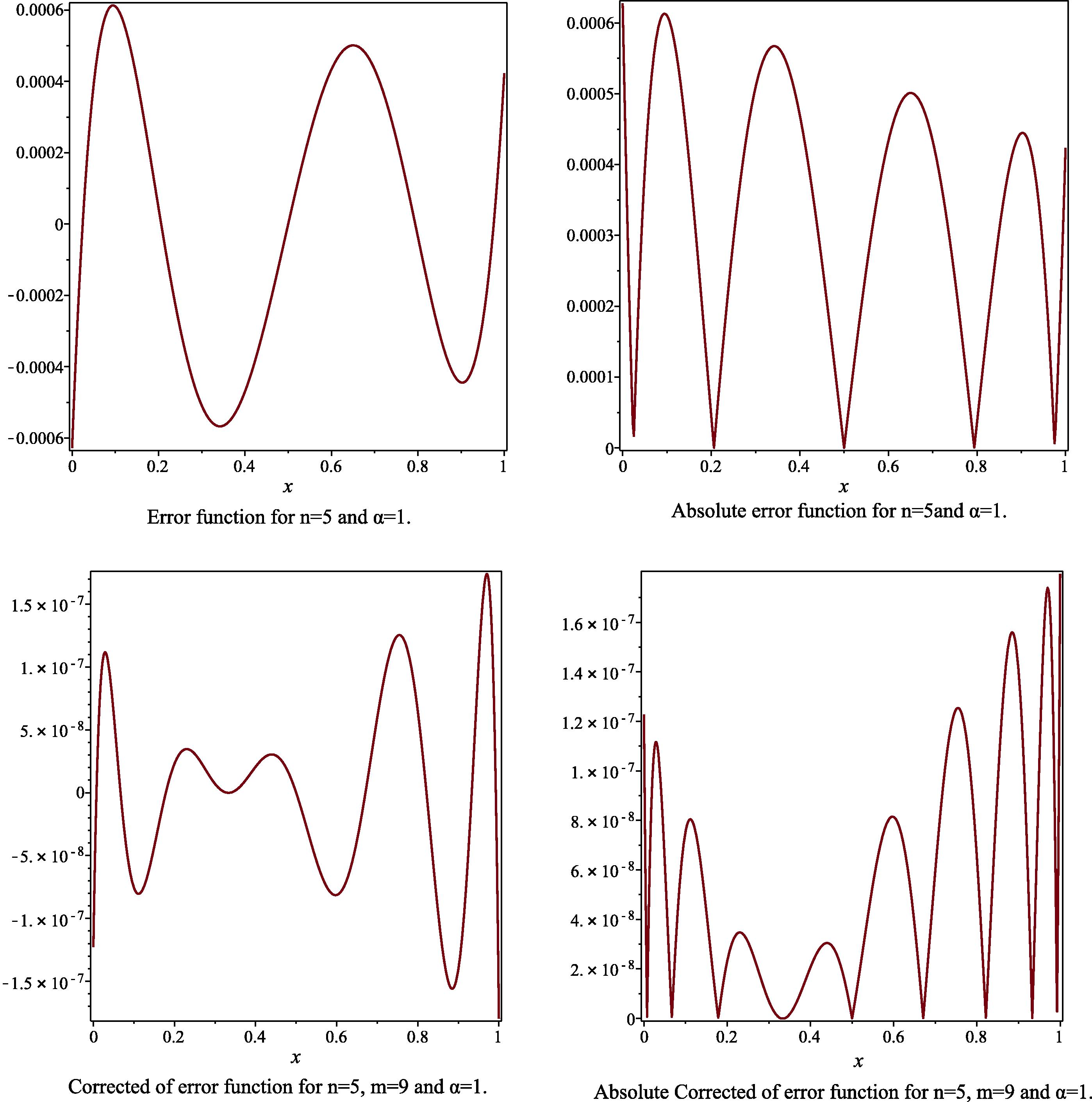
- The error function, the absolute of error function, the corrected error function and the absolute corrected error function to Example 2, for the case
- The error function, the absolute of error function, the corrected error function and the absolute corrected error function to Example 2, for the case
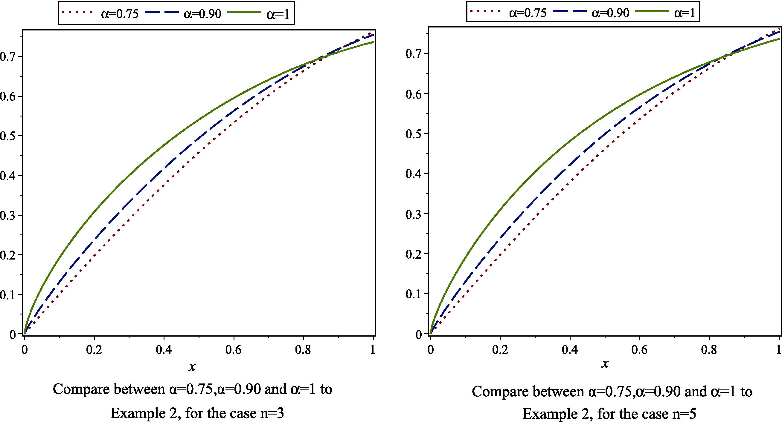
- Compare between
- The error function, the absolute of error function, the corrected error function and the absolute corrected error function to Example 3, for the case
- The error function, the absolute of error function, the corrected error function and the absolute corrected error function to Example 3, for the case
- The error function, the absolute of error function, the corrected error function and the absolute corrected error function to Example 3, for the case
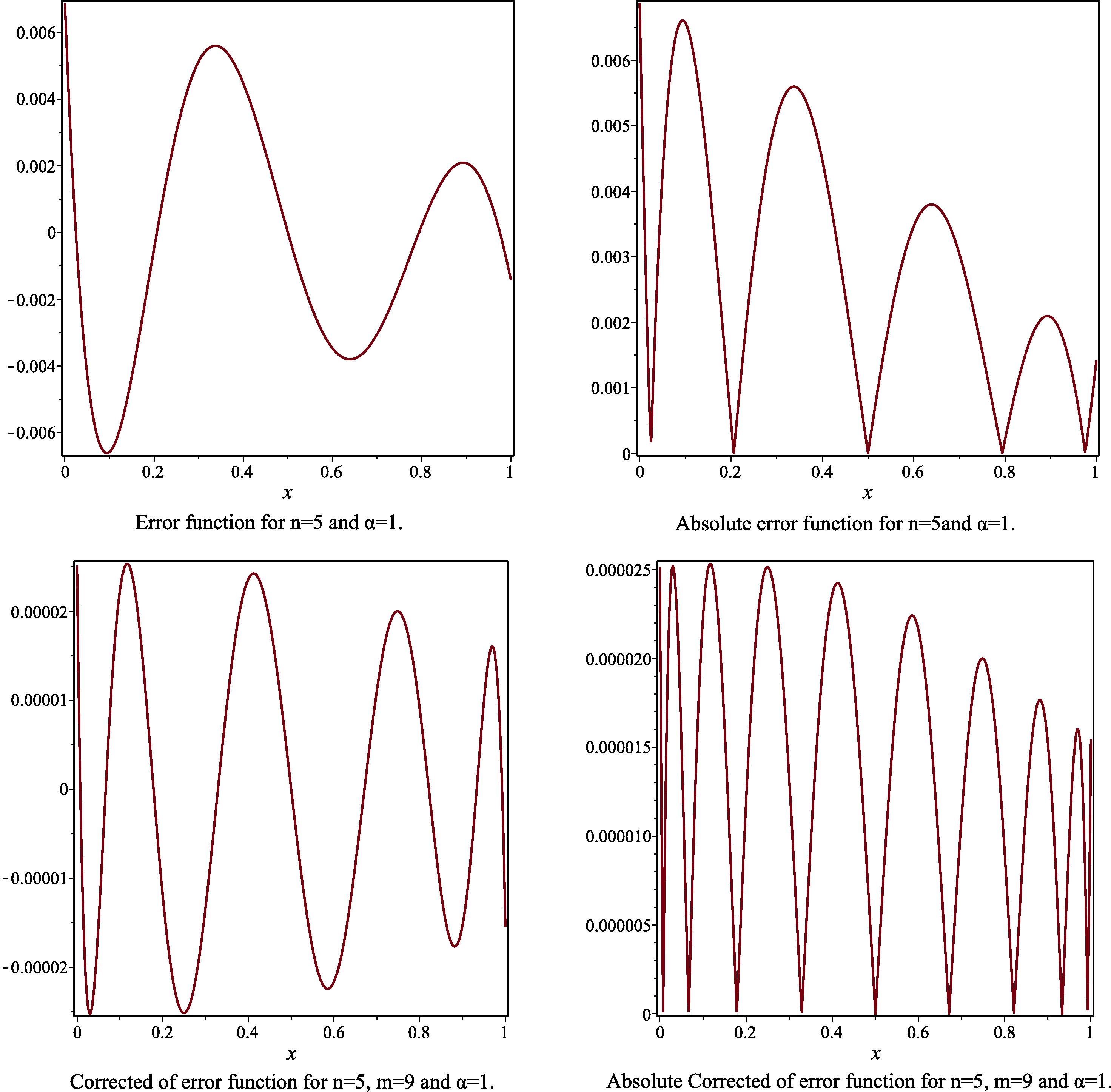
- The error function, the absolute of error function, the corrected error function and the absolute corrected error function to Example 3, for the case
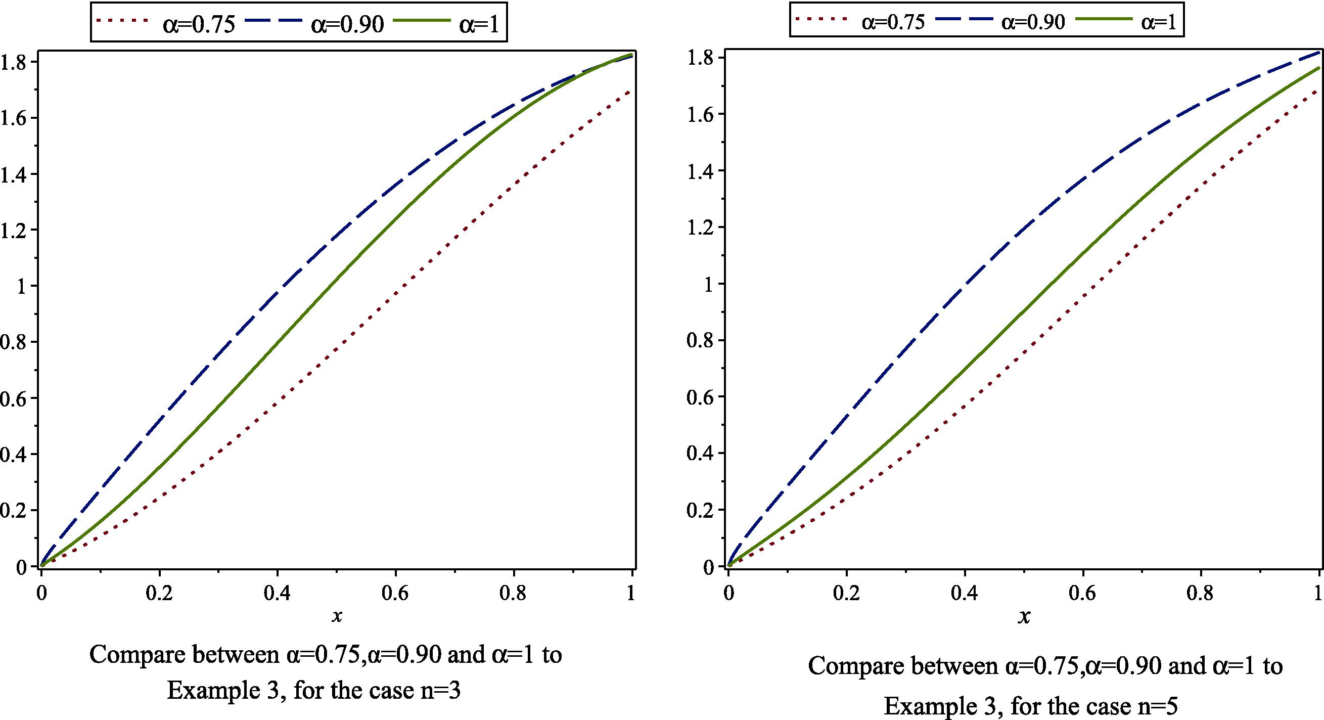
- Compare between
6 Conclusions
In this paper, the Bernstein operational matrix of derivative was applied to solve linear and non-linear fractional differential equations. Different from other numerical techniques, the few
References
- New ultraspherical Wavelets spectral solutions for fractional Riccati differential equations. Abst. Appl . Anal.. 2014;2014:Art. ID 10853375
- [Google Scholar]
- Solving system of fractional differential equations by homotopy perturbation method. Phys. Lett. A. 2008;372(4):451-459.
- [Google Scholar]
- Multistage Bernstein polynomials for the solutions of the Fractional Order Stiff Systems. J. King Saud Univ.. 2016;28:280-285.
- [Google Scholar]
- Solutions of differential equations in a Bernstein polynomial basis. Comp. Appl. Math.. 2007;189:541-548.
- [Google Scholar]
- Collocation method and residual correction using Chebyshev series. Appl. Math. Comput.. 2006;174:910-920.
- [Google Scholar]
- The solution of the Bagley–Torvik equation with the generalized Taylor collocation method. J. Frank. Inst.. 2010;347:452-466.
- [Google Scholar]
- Solving a multi-order fractional differential equations using adomian decomposition. Appl. Math. Comput.. 2007;189:541-548.
- [Google Scholar]
- Algorithms for the fractional calculus: a selection of numerical methods. Comp. Methods Appl. Mech. Eng.. 2005;194:743-773.
- [Google Scholar]
- Solving a multi-order fractional differential equations using adomian decomposition. Appl. Math. Comput.. 2007;189(1):541-548.
- [Google Scholar]
- Using an enhanced homotopy perturbation method in fractional differential equations via deforming the linear part. Appl. Math. Comp.. 2008;56:3138-3149.
- [Google Scholar]
- Solving fractional diffusion and wave equations by modified homotopy perturbation method. Phys. Lett. A. 2007;370(5-6):388-396.
- [Google Scholar]
- An integral operational matrix based on Jacobi polynomials for solving fractional-order differential equations. Appl. Math. Modell.. 2013;37:1126-1136.
- [Google Scholar]
- Fractional-order Legendre functions for solving fractional-order differential equations. Appl. Math. Modell.. 2013;37:5498-5510.
- [Google Scholar]
- An Introduction to the Fractional Calculus and Fractional Differential Equations. New York, USA: Wiley-Interscience, John Wiley and Sons; 1993.
- Decomposition method for solving fractional Riccati differential equations. Appl. Math. Comput.. 2006;182:1083-1092.
- [Google Scholar]
- Application of variational iteration method to nonlinear differential equations of fractional order. Int. J. Nonlinear Sci. Numer. Simul.. 2006;7:271-279.
- [Google Scholar]
- Modified homotopy perturbation method: application to quadratic Riccati differential equations of fractional order. Chaos, Solitons Fractals. 2008;36:167-174.
- [Google Scholar]
- Solution of Lane–Emden type equations using Bernstein operational matrix of differentiation. New Astron.. 2012;17:303-308.
- [Google Scholar]
- Fractional Differential Equations. New York, USA: Academic Press; 1999.
- Numerical solution of fractional differential equations with a Tau method based on Legendre and Bernstein polynomials. Math. Methods Appl. Sci.. 2014;37:329-342.
- [Google Scholar]
- Solving fractional partial differential equations by an efficient new basis. Int. J. Appl. Math. Comp.. 2013;5:6-21.
- [Google Scholar]
- A new operational matrix for solving fractional-order differential equations. Comput Math with Appl.. 2010;59:1326-1336.
- [Google Scholar]
- Local Fractional Integral Transforms and their Applications. Academic Press, Elsevier; 2015.
- Numerical solution for the variable order time fractional diffusion equation with Bernstein polynomials. Appl. Math. Comput.. 2014;97:81-100.
- [Google Scholar]
- Operational matrices of Bernstein polynomials and their applications. Int. J. Syst. Sci.. 2010;41:709-716.
- [Google Scholar]
- Numerical solution of fractional Riccati type differential equations by means of the Bernstein polynomials. Appl. Math. Comput.. 2013;219:6328-6343.
- [Google Scholar]


