

Translate this page into:
Solitary solutions to a metastasis model represented by two systems of coupled Riccati equations
⁎Corresponding author. inga.timofejeva@ktu.edu (I. Timofejeva)
-
Received: ,
Accepted: ,
This article was originally published by Elsevier and was migrated to Scientific Scholar after the change of Publisher.
Peer review under responsibility of King Saud University.
Abstract
Solitary solutions to a two-tumor metastasis model represented by a system of multiplicatively coupled Riccati equations are considered in this paper. The interaction between tumors is modelled by a one-sided diffusive coupling when one coupled Riccati system influences the other, but not the opposite. Necessary and sufficient conditions for the existence of solitary solutions to the composite system of Riccati equations are derived in the explicit form. Computational experiments are used to demonstrate the transitions from one steady-state to another via non-monotonous trajectories.
Keywords
Nonlinear differential equation
Analytical solution
Tumor model
35C08
34A25
92C50

1 Introduction
Mathematical modeling of biomedical processes, and cancer, in particular, has come to the forefront of research in recent decades (Altrock et al., 2015). A conceptual framework for cancer biology aims to identify the structure, the dynamics, and the rules governing the regulation of the behavior of the system (Medina, 2018).
A vast plethora of cancer models have been introduced into the scientific literature during the last years (Magi et al., 2017). In general, these models can be classified according to the mathematical modeling approach: the top-down approach and the bottom-up approach (Shahzad and Loor, 2012). Also, mathematical models of cancer are built at different scales with different degrees of detail (Medina, 2018): very detailed models of metabolic pathways, middle scale models based on fluxomics, and global phenomenological scale cancer models based on the interaction of populations of cells.
Global phenomenological scale cancer modeling approaches can be characterized either as continuous models or discrete models (with various subclasses under each type) (Simmons et al., 2017). Continuum models generate solutions as concentrations of different types of cells. Usually, they comprise a system of differential equations (though agent-based, multi-scale, lattice-based, image-based models are widely used also) (Simmons et al., 2017). Ordinary differential equations are employed if the variation of cell populations is investigated in time. Partial differential equations are employed to describe the variation both in time and in space.
Mathematical models of a single cancer tumor comprising a system of two ordinary differential equations coupled by multiplicative terms are widely used for the phenomenological description of the interaction between healthy and cancer cells (Liu and Yang, 2016). Such types of models comprising two Riccati type nonlinear coupled differential equations are used for the description of prostate cancer treatment with androgen deprivation therapy (Zazoua and Wang, 2019), cancer stem cell-targeted immunotherapy (Sigal et al., 2019; Alqudah, 2020), the maximization of viability time in general cancer therapy (Bratus et al., 2017).
The phenomenological model of such systems in mathematical terms reads:
A formal classification of multiple cancers in humans is first done in Moertel (1977). According to this classification, multiple primary cancers of the first type occur in organs with the same histology. The second type of multiple primary cancers originate from different tissues or organs. The third type of multiple cancers comprise three or more cancers at different tissues and organs that concurrently coexist with the first type of cancers (Moertel, 1977). Cancers of the first type are further subdivided into three groups: 1A – two or more cancers that occur in the same tissue or organ; 1B – cancers in a joint tissue shared by different organs; 1C – cancers occurring in bilaterally paired organs (Moertel, 1977).
Multiple primary cancers (MPC) are classified as synchronous and metachronous cancers (Jena et al., 2016). Among patients with MPC, triple cancers occur in 0.5 %, and quadruple or quintuple cancers in less than 0.1 % of the population (Kim et al., 2010; Kim et al., 2013). For metachronous gastric cancer patients, the most common cancer sites are: colorectum, thyroid, lung, kidney, and breast (in descending order) (Kim et al., 2013). For synchronous gastric cancer, a different order is observed: head and neck, esophagus, lung, and kidney (Kim et al., 2013). Females are at a higher risk of being diagnosed with a first primary cancer of breast or thyroid cancer at a younger age – but those who survived their first primary cancer are at a higher risk of developing a metachronous second primary cancer after that (Jena et al., 2016).
The life expectancy for a person diagnosed with multiple cancer is significantly shorter compared to a person only with a single isolated cancer (Jena et al., 2016). For instance, MPC developed in 10.4% of patients during five years after stomach cancer treatment (Jena et al., 2016). The probability of survival of such patients with MPC was considerably less than of patients with only a single stomach cancer (Jena et al., 2016). The majority of patients with synchronous MPC died during two years after the removal of the stomach. The survival rate of patients with metachronous MPC was also low – but many of those patients did survive for five years. The percentages of patients who did survive for five years after the removal of the stomach where: 76.5% for patients without MPC; 67.5% for patients with metachronous MPC; 34.1% for patients with synchronous MPC (Jena et al., 2016).
A mathematical model for the immune-mediated theory of metastasis is recently presented in Rhodes and Hillen (2019). The interaction between different tumors is modelled by using diffusive terms representing the migration of cancer cells between primary and secondary tumors in Rhodes and Hillen (2019). This corresponds well to the mathematical model of migration in diffusively coupled prey-predator system on heterogenous oriented graphs (Nagatani, 2020).
The main objective of this paper is to explore the existence of solitary solutions in a paradigmatic cancer metastasis model where the model of a single tumor is represented by a system of coupled ordinary differential equations with multiplicative terms, and the interaction between primary and secondary tumors is represented by a diffusive term.
In mathematical terms, this model can be represented by the following system of nonlinear differential equations:
This model uses a system of coupled Riccati type differential equations to characterize the dynamics of a single tumor (Liu and Yang, 2016; Zazoua and Wang, 2019; Sigal et al., 2019; Alqudah, 2020; Bratus et al., 2017). On the other hand, the diffusive terms coupling different tumors fall in line with the model of metastasis presented in Rhodes and Hillen (2019). Moreover, Eq. (2) does generalize the model of diffusively coupled prey-predator system on heterogenous graphs (Nagatani, 2020) because the governing differential equations representing the dynamics of healthy and cancer cells in each tumor are nonlinear Riccati differential equations (linear differential equations are used in Nagatani (2020)). The model presented by Eq. (2) also can be interpreted as the phenomenological generalization of the Master–Slave model comprising two discrete logistic maps (Ramirez et al., 2018). The dissipative coupling between different tumors is a one-way coupling. In other words, the primary (the “Master”) tumor does have a direct impact on the growth of the secondary (the “Slave”) tumor, but not vice versa. As mentioned previously, such dissipative connection between tumors does represent the model of the metastasis discussed in Rhodes and Hillen (2019).
Such kind of generalization of the metastasis model on heterogenous graph poses an important theoretical challenge from the mathematical point of view. The existence of solitary solutions in an androgen-deprivation prostate cancer treatment model (Telksnys et al., 2020), a hepatitis C evolution model (Telksnys et al., 2018), or a model of a biological neuron (Telksnys et al., 2019) always allows to construct the global view of the system dynamics in the phase space of system parameters and initial conditions. The matter of fact is, that solitary solutions to these models do usually represent separatrix between different basin boundaries (Telksnys et al., 2019; Telksnys et al., 2018; Telksnys et al., 2020). Therefore, the ability to identify solitary solutions (and the corresponding basin boundaries) would provide an important insight into the dynamics of the paradigmatic cancer metastasis model.
2 Preliminaries
2.1 The concept of solitary solutions
Analytical functions of the form:
The substitution:
2.2 The inverse balancing technique
The primary question that has to be answered when considering solitary solutions to a particular system is whether they exist as solutions, and if so, what conditions must the system parameters and solution parameters satisfy. The inverse balancing technique, presented in detail in Navickas et al. (2016), given a system or differential equations, both determines the maximum solitary solution order and derives the necessary and sufficient conditions for their existence.
The fundamental idea of the technique is to insert the expression (5) as the ansatz into the system of differential equations. After simplifying, a linear system of equations with respect to the equation parameters is obtained. The conditions under which this system is non-singular coincide with the necessary existence solutions for the solitary solutions.
This approach differs significantly from the direct construction: in the latter, after inserting the ansatz into the system of differential equations, the resulting nonlinear equations are solved for the solution, rather than the system parameters. This yields a high-order system of equations that cannot always be solved, especially if all solutions are to be obtained. Due to these complications, we forgo the direct approach and use the inverse balancing technique to analyze (2).
3 Existence of solitary solutions in the Riccati system
The substitution (4) can be used on (2), resulting in:
For the derivations presented, the following functions have to be defined:
Inserting the ansatz (11)–(12) into (7)–(10) yields:
The first two equations can be multiplied by
and
, respectively; the last two by T, resulting in a simplified version of (20)–(23):
Each of the above equations can only hold if both right and left terms are polynomials of order n, which means the left side denominators must cancel out in each case:
The above relations coincide with the necessary existence conditions for solitary solutions to (2). They can be further simplified as:
Combining (28)–(31) with (24)–(27) results in:
Obtained Eqs. (36)–(39) are sufficient conditions for solutions (11) to exist in the system (2). These conditions can be further rearranged:
4 Maximum possible order of solitary solutions to the Riccati system
The inverse balancing technique, discussed in detail in Section 2.2, is used to determine the maximum possible order solitary solutions to the considered Riccati system (2).
The following isomorphisms are introduced:
Applying the above identities, previously derived conditions (32)–(35) and (40)–(43) can be restated via the defined vectors:
All of the parameters defined above can be placed in one of three exclusive groups which can be represented by a schematic diagram in Fig. 1:
-
and are parameters of the Riccati system (2).
-
and where are parameters of the solitary solutions.
-
and , where are auxiliary parameters that neither belong to the solution nor the system of differential equations. The first two, and , are applied in the derivation of conditions (54)–(57) (specifically (28)–(31)). The remaining parameters relate the Riccati system and its solitary solution parameters via necessary and sufficient conditions (54)–(57).
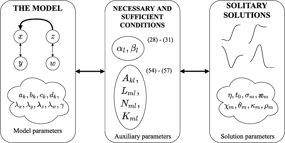
- A schematic diagram portraying the relationship between different groups of parameters.
The solitary solution and auxiliary parameters can be derived as a solution to the algebraic Eqs. (54)–(57). The Riccati system parameters are then obtained as:
Similarly to (60), using (44)–(49) in conjunction with (55) yields the following set of linear equations with
as unknowns:
Let:
Note that if
, the last two equations of (63) become identities. Otherwise, cancelling
from the last two equations of (63) results in:
Applying (44)–(49)–(56) yields another set of linear equations with unknowns
:
Finally, applying (44), (46), (48), (51) and (53)–(57) results in a set of linear equations with respect to
and
:
4.1 First order solitary solutions to (2)
First order solitary solutions (kink solutions) will be considered in this subsection. The selection
transforms systems (65), (66) into a singular form; the solutions in terms of
read:
The system (67) yields the expressions for
:
The Riccati system (2) admits the first order solitary solutions (kink solutions, ) without any constraints on Riccati system parameters or solitary solution parameters.
4.2 Higher order solitary solutions to (2)
Higher order solitary solutions are obtained by selecting
. In this case (65), (66) are no longer singular and can only admit one solution:
As shown above, in the case of higher order solitary solutions, the auxiliary parameters
and
must be equal. Thus, inserting
(
into (58) results in the following constraints on the Riccati system parameters:
Applying analogous reasoning used for the derivation of conditions (72)–(73) earlier, it could be concluded that solutions (70) to the system (67) hold if and only if the following relationships are true:
The results of the analysis performed in this subsection are summarized in the following Lemma.
The Riccati system (2) admits higher order solitary solutions ( ) if and only if (72), (74) and (75)–(76) do hold true.
4.3 The algebraic structure of higher order solitary solutions ( )
The solutions (11)–(12) can be rewritten in a different form considering (61)–(62) and (64):
It is important to note that necessary and sufficient conditions mentioned in Lemma 4.1 do result in a specific algebraic structure of higher order solitary solutions. The following Lemma splits the family of solutions into two cases.
While the Riccati system (2) can admit solitary solutions of arbitrary order, some solutions may have constraints imposed on their parameters:
Note that case (ii) of the above Lemma does not inherently mean that higher order solitary solutions become more complex: due to the result that parameters must be set to zero, these solutions retain a maximum number of two extrema.
5 Numerical experiments
5.1 Kink solitary solution to a single Riccati equation
Consider the following Riccati equation:
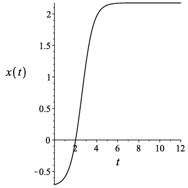
Kink solitary solution
to (81).
5.2 Bright/dark solitary solutions to a system of Riccati equations with multiplicative coupling
Consider the following system of Riccati equations with multiplicative coupling:
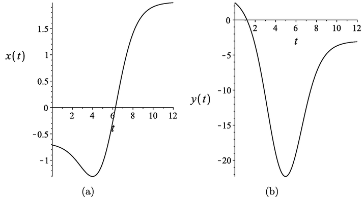
Bright/dark solitary solutions
(part (a)) and
(part (b)) to (82)–(83).
5.3 Second order solitary solutions to the system (2)
Suppose the following Riccati system is given:
Firstly, solitary solution parameters
(
),
and
are selected as follows:
Then, the auxiliary parameters
and
(
) are computed from (58):
Having derived the auxiliary parameters, it is now possible to use (61)–(62), (70), (71) and (75)–(76) to obtain the missing solitary solution parameters
and
(
):
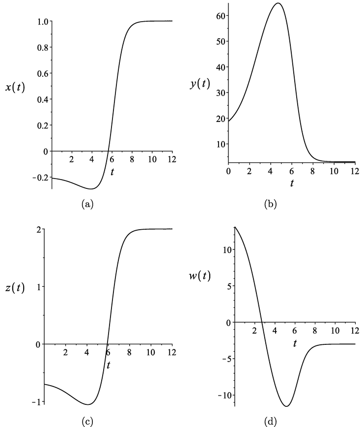
The above parameters yield the following non-singular second order solitary solutions:
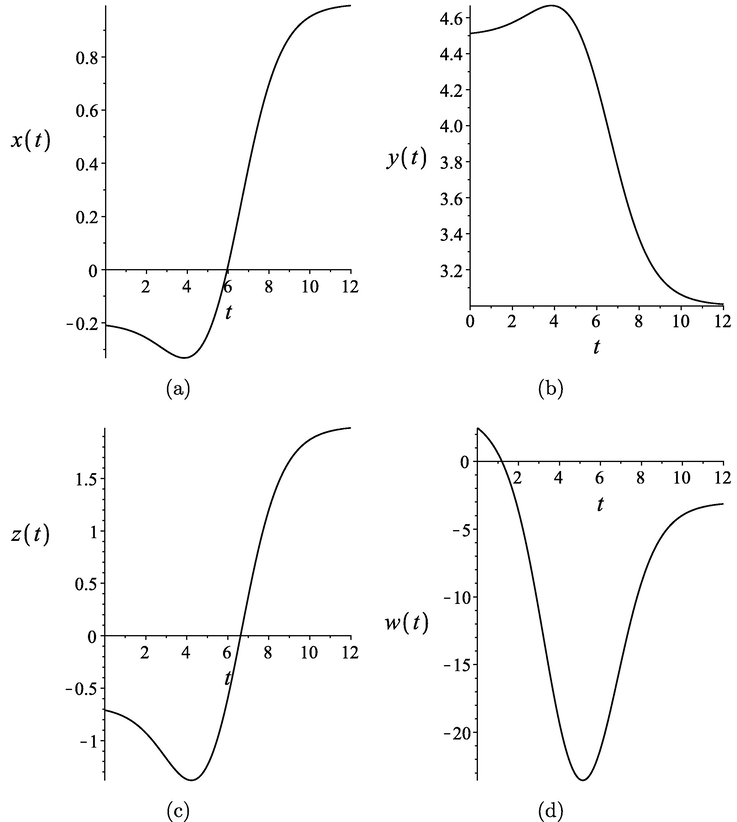
Second order solitary solutions
(part (a)),
(part (b)),
(part (c)) and
(part (d)) to (84)–(87).
5.4 Third order solitary solutions to the system (2)
In this subsection, the third order solitary solutions (
) are constructed for the following Riccati system:
Analogously as in the previous subsection, solitary solution parameters
(
),
and
are selected as follows:
From the Lemma 4.2 it follows that .
The auxiliary parameters
and
(
) are then obtained from (58):
Finally, the solitary solution parameters
and
(
) are computed using (61)–(62), (70), (71) and (75)–(76):
Thus, the Riccati system (95)–(98) admits the following non-singular third order solitary solutions:
Third order solitary solutions
(part (a)),
(part (b)),
(part (c)) and
(part (d)) to (95)–(98).
6 Conclusions
Solitary solutions to model (2), representing cancer metastasis, were derived in this paper. Note that (2) represents a system with a one-way interaction between tumors: both tumor nodes are represented via Riccati systems with multiplicative coupling, however, the first node is autonomous (in the sense that it is not influenced by the remainder of the system), and the second is diffusively coupled with the first. This results in a system where the inter-node interactions are represented by a single diffusive term, rather than a two-way interaction consisting of two terms, discussed in detail in Telksnys et al. (2020).
While system (2) may appear similar to the Riccati system discussed in Telksnys et al. (2020), their dynamics are distinct. In either case, the evolution of tumor cell populations is non-monotonous, possessing both maxima and minima for finite time values as well as differing ratios of limits as time tends to or . However, with a single diffusive term, as discusssed in this paper, solitary solutions with at most two maxima (irregardles of the actual order n of the solution) can be obtained, while two diffusive terms in the analogous system results in at most three maxima.
Furthermore, it can be noted that the relation between cell population in the nodes themselves can be representative of tumor evolution: functions evolve from a higher steady-state to a lower one, while do the opposite. It is interesting to observe that the androgen-deprivation prostate cancer treatment model does admit only bright/dark (the second order) solitary solutions (Telksnys et al., 2020) However, this paper shows that the order of solitary solutions admitted by the metastasis model represented by multiplicatively and diffusively coupled Riccati systems can be larger than two. Together with the results of Telksnys et al. (2020), this paper provides a comprehensive study on solitary solutions to tumor models. Extensions of these models containing more complex coupling terms (both inside the nodes and between them) remain a definite objective of future research.
Declaration of Competing Interest
The authors declare that they have no known competing financial interests or personal relationships that could have appeared to influence the work reported in this paper.
References
- Alqudah, M.A., 2020. Cancer treatment by stem cells and chemotherapy as a mathematical model with numerical simulations, Alexandria Eng. J.
- The mathematics of cancer: integrating quantitative models. Nat. Rev. Cancer. 2015;15(12):730-745.
- [Google Scholar]
- Maximization of viability time in a mathematical model of cancer therapy. Mathe. Biosci.. 2017;294:110-119.
- [Google Scholar]
- Clinicopathologic features of metachronous or synchronous gastric cancer patients with three or more primary sites. Cancer Res. Treat.: Off. J. Korean Cancer Assoc.. 2010;42(4):217.
- [Google Scholar]
- Prediction of metachronous multiple primary cancers following the curative resection of gastric cancer. BMC Cancer. 2013;13(1):394.
- [Google Scholar]
- A mathematical model of cancer treatment by radiotherapy followed by chemotherapy. Mathe. Comput. Simul.. 2016;124:1-15.
- [Google Scholar]
- Current status of mathematical modeling of cancer–from the viewpoint of cancer hallmarks. Curr. Opin. Syst. Biol.. 2017;2:39-48.
- [Google Scholar]
- Mathematical modeling of cancer metabolism. Crit. Rev. Oncol./Hematol.. 2018;124:37-40.
- [Google Scholar]
- Multiple primary malignant neoplasms. historical perspectives. Cancer. 1977;40(S4):1786-1792.
- [Google Scholar]
- Migration difference in diffusively-coupled prey–predator system on heterogeneous graphs. Physica A. 2020;537:122705
- [Google Scholar]
- Existence of solitary solutions in a class of nonlinear differential equations with polynomial nonlinearity. Appl. Math. Comput.. 2016;283:333-338.
- [Google Scholar]
- Existence of second order solitary solutions to riccati differential equations coupled with a multiplicative term. IMA J. Appl. Mathe.. 2016;81(6):1163-1190.
- [Google Scholar]
- Handbook of Nonlinear Partial Differential Equations. CRC Press; 2004.
- Enhancing master-slave synchronization: The effect of using a dynamic coupling. Phys. Rev. E. 2018;98(1):012208
- [Google Scholar]
- A mathematical model for the immune-mediated theory of metastasis. J. Theoret. Biol.. 2019;482:109999
- [Google Scholar]
- Application of top-down and bottom-up systems approaches in ruminant physiology and metabolism. Curr. Genomics. 2012;13(5):379-394.
- [Google Scholar]
- Mathematical modelling of cancer stem cell-targeted immunotherapy. Math. Biosci.. 2019;318:108269
- [Google Scholar]
- Environmental factors in breast cancer invasion: a mathematical modelling review. Pathology. 2017;49(2):172-180.
- [Google Scholar]
- Homoclinic and heteroclinic solutions to a hepatitis c evolution model. Open Mathe.. 2018;16(1):1537-1555.
- [Google Scholar]
- Symmetry breaking in solitary solutions to the hodgkin–huxley model. Nonlinear Dyn.. 2019;97(1):571-582.
- [Google Scholar]
- Solitary solutions to an androgen-deprivation prostate cancer treatment model. Mathe. Methods Appl. Sci.. 2020;43(7):3995-4006.
- [Google Scholar]
- Analysis of mathematical model of prostate cancer with androgen deprivation therapy. Commun. Nonlinear Sci. Numer. Simul.. 2019;66:41-60.
- [Google Scholar]


