Sharp bounds on partition dimension of hexagonal Möbius ladder

Muhammad Azeem; Muhammad Imran; Muhammad Faisal Nadeem

doi:10.1016/j.jksus.2021.101779

View/Download PDF

Sharp bounds on partition dimension of hexagonal Möbius ladder

Muhammad Azeem^{^a}, Muhammad Imran^{^b,⁎}, Muhammad Faisal Nadeem^{^c}

a Department of Aerospace Engineering, Faculty of Engineering, University Putra Malaysia, Malaysia

b Department of Mathematical Sciences, United Arab Emirates University, Al Ain, United Arab Emirates

c Department of Mathematics, COMSATS University Islamabad, Lahore Campus, Lahore Pakistan

⁎Corresponding author. m.imran658@uaeu.ac.ae (Muhammad Imran),

Received: 2021-5-6, Accepted: 2021-12-16,

Disclaimer:
This article was originally published by Elsevier and was migrated to Scientific Scholar after the change of Publisher.

Peer review under responsibility of King Saud University.

Abstract

Complex networks are not easy to decode and understand to work on it, similarly, the Möbius structure is also considered as a complex structure or geometry. But making a graph of every complex and huge structure either chemical or computer-related networks becomes easy. After making easy of its construction, recognition of each vertex (node or atom) is also not an easy task, in this context resolvability parameters plays an important role in controlling or accessing each vertex with respect to some chosen vertices called as resolving set or sometimes dividing entire cluster of vertices into further subparts (subsets) and then accessing each vertex with respect to build in subsets called as resolving partition set. In these parameters, each vertex has its own unique identification and is easy to access despite the small or huge structures. In this article, we provide a resolving partition of hexagonal Möbius ladder graph and discuss bounds of partition dimension of hexagonal Möbius ladder network.

Keywords

Möbius ladder graph

Partition dimension

Partition resolving sets

Bounds of partition dimension

Show Related Articles from PubMed

1 Introduction

Hexagonal network is used in several fields of sciences, due to its advantages compared to other several lattice networks. Hexagonal networks have an uncomplicated and symmetrical adjoining neighborhood, which avoids the uncertain behavior that square or triangular networks have. When the adjacent locality, path, or connectivity is critical, the square and triangular networks are not appropriate. Current investigation on image processing and digital images discovered that using a hexagonal network as an alternative to square networks provides improved outcomes Kumar et al., 2014; Wen and Khatibi, 2018. In the area of ecology, the advantages of using hexagons are presented in observation, experiment, and simulation, with excellent benefits, provided in natural demonstrating Birch et al., 2007. Many investigators recommend the use of a hexagonal network, especially in cartography, in the order to obtain smaller resolutions by using the disintegration of the larger cells into smaller ones Mocnik, 2018; Sahr et al., 2003.

The notion of metric dimension appeared with various titles. Slater SSlater and treeslater and trees, 1975 introduced the notion of metric dimension as locating sets, later Harary and Melter Harary and Melter, 1976 proposed the idea by in terms of metric dimension instead of locating sets. Chartrand et al. Chartrand et al., 2000, described the notion of metric dimension as resolving sets. For more details on resolving set, metric basis and metric dimension appeared we refer to see Chartrand et al., 2000; Chartrand et al., 2000; Chartrand et al., 2000; J. Caceres et al., 2007; Khuller et al., 1996; Chvatal, 1983 . The generalized version of metric dimension is called partition dimension defined in Chartrand et al., 2000. The metric dimension of a connected graph is based on the distances among the vertices while the partition dimension is based on the distances among the vertices and sets containing vertices. It was proved that determining the metric dimension of a graph is a NP-hard problem Chartrand et al., 2000. Since partition dimension is a generalization of finding the metric dimension, therefore finding the partition dimension of a graph is also an NP-hard problem.

It is natural to ask about the characterizations of the graphs based on the nature of the partition dimension. Researchers are always interested to prove that whether the partition dimension of a family of a network is constant, bounded or unbounded. Therefore, the study of finding partition dimension of a graph significantly appeared and several results are found. Such as; Baskoro et al. Baskoro et al., 2020 discussed graphs with partition dimension $n - 3$ , Vertana and Kasmayadi obtained the partition dimension of graphs constructed by sum operation of cycle and path graphs Vertana and Kusmayadi, 2016, Hussain et al. Hussain et al., 2019 provide bounds of partition dimension of M-wheels, Grigorious et al. Grigorious et al., 2017, Maritz et al. Maritz and Vetrik, 2018 found the partition dimension of circulant graph, Safriadi et al. computed it for complete multipartite graph Safriadi et al., 2020, strong partition dimension discussed in Kuziak and Yero, 2020; Rehman and Mehreen, 2020 by Kuziak and Yero, Rehman and Mehreen respectively, Mehreen et al. Mehreen et al., 2018 computed the partition dimension of $(4, 6)$ fullerene, and proved that it has bounded partition dimension. Results on the bounded partition dimension of the Cartesian product of graphs are studied in Yero et al., 2010. Amrullah et al. in Amrullah et al., 2019 gave bounds for the subdivision of different graphs. Rodrı̀uez-Velàzquez, et al. Rodrł̀uez-Velàzquez et al., 2014 provide the bounds of tree graph. Rodrı̀uez-Velàzquez, et al. in Rodrł̀uez-Velàzquez et al., 2014 discussed bounds of unicyclic graphs in the form of subgraphs. Javaid et al. found the bounds on the fractional metric dimension of some networks Javaid et al., 2020. Chu et al. computed the sharp bounds for the partition dimension of convex polytopes Chu et al., 2020. For more recent literature and results, we refer to see Rodrł̀uez-Velàzquez et al., 2014; Rodrł̀uez-Velàzquez et al., 2014; Mehreen et al., 2018; Monica and Santhakumar, 2016; Rajan et al., 2012; Javaid and Shokat, 2008; Moreno, 2020; Haryeni et al., 2017 .

Applications of resolving partition parameter can be found in various fields such as network verification and its discovery Beerliova et al., 2006, Khuller et al. discussed resolving partitions in robot navigations, Caceres et al. relate the famous Djokovic-Winkler relation J. Caceres et al., 2007, and Chvatal describe the resolving sets considering as an application for the strategies of the mastermind games Chvatal, 1983. Further, applications of resolving sets can be found in Johnson, 1993; Johnson, 1998; Melter and Tomescu, 1984 . Moreover, to explore the applications of this concept in networks, we refer to see Chartrand et al., 2000; Harary and Melter, 1976. Due to vast applications of partition dimension and hexagonal networks, in this paper, we computed the partition dimension of hexagonal Möbius ladder network.

2 Preliminaries

Following are some useful mathematical notions of the ideas which help to understand the concepts required.

Definition 2.1

Let N be an undirected graph with set of vertices $V (N)$ and set of edges $E (N)$ , the distance (also known as geodesics) between $ϕ_{1}, ϕ_{2} \in V (N)$ two vertices is the minimum number of edges between $ϕ_{1} - ϕ_{2}$ path. It is represented by $d (ϕ_{1}, ϕ_{2})$ .

Definition 2.2

Let $Q = {ϕ_{1}, ϕ_{2}, \dots, ϕ_{t}}$ be an ordered subset of vertices, and $ϕ \in V (N)$ . The representations $r (ϕ | Q)$ of $ϕ$ -vertex with respect to Q is the $t$ -tuple distances $(d (ϕ, ϕ_{1}), d (ϕ, ϕ_{2}), \dots, d (ϕ, ϕ_{t}))$ . If every vertex of $V (N)$ have distinctive representation with respect to Q, then Q is said to be a resolving set of graph N, and minimum number of the vertices in Q is known as the metric dimension of graph N and it is denoted by $\dim (N)$ .

Definition 2.3

Let P be a k-ordered partition set and $r (ϕ | P) = {d (ϕ, P_{1}), d (ϕ, P_{2}), \dots, d (ϕ, P_{k})}$ , be a k-tuple distance representation of a vertex $ϕ$ regarding P. If the representation of $ϕ$ with respect to P is distinctive, then P is called the partition resolving set of graph N.

Definition 2.4

Chartrand et al., 2000 The minimum number of subsets in the partition resolving set of $V (N)$ is called the partition dimension $(pd (N))$ of N.

The $\dim (N)$ and $pd (N)$ can be related for any simple connected graph N Chartrand et al., 2000;

(1)

pd (N) ⩽ \dim (N) + 1 .

Theorem 2.5

Chartrand et al., 2000 Let P be a partition resolving set of $V (N)$ and $ϕ_{1}, ϕ_{2} \in V (N)$ . If $d (ϕ_{1}, w) = d (ϕ_{2}, w)$ for all vertices $w \in V (N) ⧹ (ϕ_{1}, ϕ_{2})$ , then $ϕ_{1}, ϕ_{2}$ belongs to different subsets of P.

Theorem 2.6

Chartrand et al., 2000 Let N be a simple and connected graph, then

$pd (N)$ is two iff N is only a path graph
$pd (N)$ is $| N |$ iff N is a complete graph.

2.1

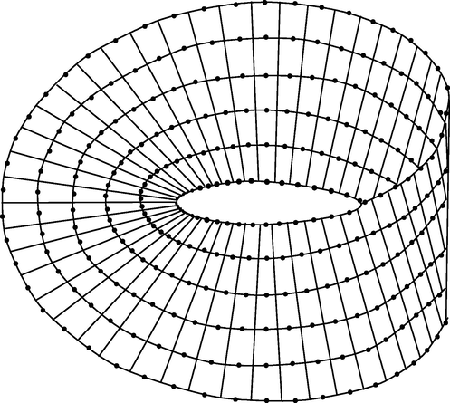
2.1 Hexagonal Möbius ladder network

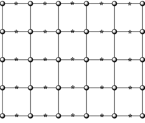
Recently, Nadeem et al. Nadeem et al., 2020 define the structure of hexagonal Möbius ladder network and computed its metric dimension. The Möbius graph is constructed by adding a vertex on each horizontal edges of square grid, as shown in Fig. 1, each cycle is order six in the grid which is the reason to called the hexagonal grid and Nadeem et al., 2020 named it hexagonal Möbius ladder graph. Twist this hexagonal grid $180 °$ which is shown in Fig. 1 and identify the utmost right and left vertices as shown in Fig. 2. The Möbius ladder graph $MG (η, ξ)$ has $ξ$ vertical and $η$ horizontal cycles. The order of $MG (η, ξ)$ is $χ = 2 η (ξ + 1)$ .

3 Main results

In this section, we determine the bounds of partition dimension of hexagonal Möbius ladder network.

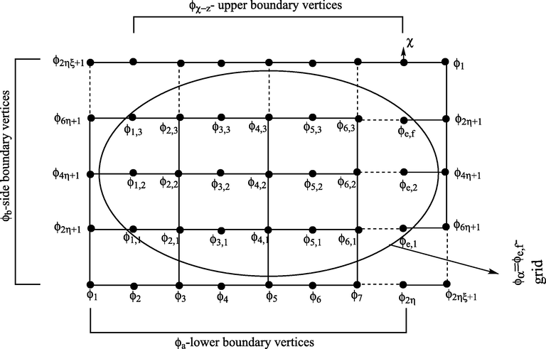
Fig. 2 is the $2 D$ -view of Möbius ladder, we label the lower boundary vertices $ϕ_{a}$ where $1 ⩽ a ⩽ 2 η$ , the side boundary vertices $ϕ_{b}$ where $b = 2 η f + 1$ and $1 ⩽ f ⩽ η$ , upper boundary vertices $ϕ_{χ - z}$ where $χ = 2 η (ξ + 1)$ and $0 ⩽ z \leq 2 η - 2$ , and lastly, the grid vertices $ϕ_{e, f} = ϕ_{α}$ where ${e, f} = α = 2 η f + e + 1$ , and $1 ⩽ f ⩽ ξ - 1, 1 ⩽ e ⩽ η - 1$ . Fig. 3 displays a three dimensional view of $MG (η, ξ)$ .

Example 3.1

The partition dimension of $MG (2, 1)$ is three. To show this, let $P = {P_{1}, P_{2}, P_{3}} = V (MG (2, 1))$ , where $P_{1} = {ϕ_{2}}, P_{2} = {ϕ_{4}}$ and $P_{3} = V (MG (2, 1)) ⧹ {ϕ_{2}, ϕ_{4}}$ be a partition resolving set, different representations of all the vertices of $MG (2, 1)$ with respect to its partition resolving set P are shown in Table 1.

We can see that all the vertices have unique representations with respect to the partition resolving set P. Hence, $pd (MG (2, 1)) = 3$ .

Möbius ladder graph MG ( η , ξ ) 3D view.

Table 1 Representations of the vertex set

ϕ_{a}

w.r.t P.

$d (., .)$	$P_{1}$	$d (., .)$	$P_{2}$	$d (., .)$	$P_{3}$
$ϕ_{a} : a = 1, 3$	1	$ϕ_{a} : a = 3, 5$	1	$ϕ_{a} : a = 1, 3, 5, 6, 7, 8$	0
$ϕ_{a} : a = 4, 5, 7, 8$	2	$ϕ_{a} : a = 1, 2, 6, 7$	2	$ϕ_{a} : a = 2, 4$	1
$ϕ_{a} : a = 6$	3	$ϕ_{a} : a = 8$	3

Now, we will find the bounds of partition dimension of $MG (η, ξ)$ , for different variations of $η$ and $ξ$ .

Theorem 3.2

If $MG (η, ξ)$ is a hexagonal Möbius ladder of order $2 η (ξ + 1)$ , then $pd (MG (η, ξ)) \leq 4,$ for $η ⩾ 2$ , and $ξ ⩾ 1$ odd.

Proof

Assume the partition resolving set $P = {P_{1}, P_{2}, P_{3}, P_{4}}$ , where $P_{1} = {ϕ_{1}}, P_{2} = {ϕ_{3}}, P_{3} = {ϕ_{2 η ξ + 1}}$ and $P_{4} = V (MG (η, ξ)) ⧹ {ϕ_{1}, ϕ_{3}, ϕ_{2 η ξ + 1}}$ . Then the representations of the each elements of vertex set of $MG (η, ξ)$ with the set P are given in Eq. 2.

(2)

\begin{matrix} r (ϕ_{a} | P) = (d (ϕ_{a}, P_{1}), d (ϕ_{a}, P_{2}), d (ϕ_{a}, P_{3}), d (ϕ_{a}, P_{4})) \\ a = 1, 2, \dots, 2 η (ξ + 1) \end{matrix}

Now, we split the vector shown in Eq. (2) into components. Representations of the first component are given in Equations (3)–(7), second in Equations (8)–(12), third in Equations (13)–(17) and the last component in Eq. (18).

The distance of lower boundary vertices $ϕ_{a}$ with $P_{1}$ are:

(3)

d (ϕ_{a}, P_{1}) = \{\begin{matrix} a - 1, & 2 ⩽ a ⩽ η + ⌈\frac{ξ}{2}⌉; \\ η + ⌊\frac{ξ}{2}⌋ - g + 1, & η + ⌈\frac{ξ}{2}⌉ + g ⩽ a ⩽ 2 η, g = 1, 2, \dots, | a | . \end{matrix}

The distance of side boundary vertices $ϕ_{b}$ with $P_{1}$ are:

(4)

d (ϕ_{b}, P_{1}) = \{\begin{matrix} f, & if 1 ⩽ f ⩽ ξ for η > ξ, \\ and 1 ⩽ f ⩽ ξ - 1, for η ⩽ ξ; \\ 2 η, & if f = η and η ⩽ ξ . \end{matrix}

Here, $b = 2 η f + 1$ .

The distance of upper boundary vertices $ϕ_{χ - z}$ with $P_{1}$ are:

(5)

d (ϕ_{χ - z}, P_{1}) = \{\begin{matrix} z + 1, & if 0 ⩽ z ⩽ 2 η - 2 for η < ξ, \\ and 0 ⩽ z ⩽ η + ⌊\frac{ξ}{2}⌋ - 1, for η ⩾ ξ; \\ ξ + z, & if η ⩾ ξ . \end{matrix}

To show the distance of inner vertices $ϕ_{α} = ϕ_{e, f}$ , where $α = 2 η f + e + 1$ of the grid with $P_{1}$ , we split it into two cases:

If $η ⩾ ξ$ and $f = 1, 2, \dots, ξ - 1$ , then

(6)

d (ϕ_{α}, P_{1}) = \{\begin{matrix} ξ - 1 + e, & if 1 ⩽ e ⩽ η - f + ⌊\frac{ξ}{2}⌋; \\ η + ξ - g - 1, & if η - f + ⌊\frac{ξ}{2}⌋ + g ⩽ e ⩽ 2 η - 1, g = 1, 2, \dots, | e | . \end{matrix}

If $η < ξ$ , and $f ⩾ ξ - 2 η > 0$ , then

(7)

d (ϕ_{α}, P_{1}) = \{\begin{matrix} ξ + e, & if 1 ⩽ e ⩽ 2 η - 1 - g; \\ ξ - f + 2 η - 1, & if 2 η - g + l - 1 ⩽ e ⩽ 2 η - 1 . \end{matrix}

In this case $g = 1, \dots, 2 η - 1$ and $l = 1, \dots, η$ .

Similarly, we have the distances of all vertices with the $P_{2}$ are:

(8)

d (ϕ_{a}, P_{2}) = \{\begin{matrix} a - 3, & 4 ⩽ a ⩽ η + ⌈\frac{ξ + 1}{2}⌉; \\ α + ξ + 3 - g, & η + ⌈\frac{ξ + 1}{2}⌉ + g + 2 ⩽ a ⩽ 2 η, g = 1, \dots, | a |; \\ \frac{2}{a}, & a = 1, 2 . \end{matrix}

(9)

d (ϕ_{b}, P_{2}) = \{\begin{matrix} 2 + f, & if 1 ⩽ f ⩽ ξ for η ⩾ ξ \\ and 1 ⩽ f ⩽ η + ⌊\frac{ξ}{2}⌋ - 2 for η < ξ; \\ 2 η - 2 + f, & if η + ⌊\frac{ξ}{2}⌋ - 1 ⩽ g ⩽ ξ, f = 0, \dots, | g | for η < ξ . \end{matrix}

(10)

d (ϕ_{χ - z}, P_{2}) = \{\begin{matrix} ξ + 1, & if z = 1, 3 for η < ξ ⩽ 2 η and η > ξ; \\ ξ, & if z = 2 for η < ξ ⩽ 2 η and η > ξ; \\ z + 3, & if 0 ⩽ z \leq 2 η - 5 for η < ξ ⩽ 2 η and 0 ⩽ z ⩽ 2 η - 1 for η < ξ ⩽ 2 η; \\ also if 0 ⩽ z ⩽ η - 2 + ⌊\frac{ξ - 1}{2}⌋; \\ ξ + 1 + g, & if η - 1 + ⌊\frac{ξ - 1}{2}⌋ ⩽ z ⩽ 2 η - 4, where g = 1, \dots, |η - 2 + ⌊\frac{ξ - 1}{2}⌋| . \end{matrix}

Again for the inner grid vertices, we split into two cases;

If $η ⩾ ξ$ and $1 ⩽ f ⩽ ξ - 1$ , then

(11)

d (ϕ_{α}, P_{2}) = \{\begin{matrix} f + e, & if e = 1, 3; \\ f, & if e = 2; \\ e + f - 2, & if 4 ⩽ e ⩽ η - f + 3; \\ e + f - g, & if η - f + g + 3 ⩽ e ⩽ 2 η - 1 where g = 1, \dots, η - 4 + f . \end{matrix}

If $η < ξ$ , then

(12)

d (ϕ_{α}, P_{2}) = \{\begin{matrix} | f | + 2 + l, & if η + 4 + g ⩽ f ⩽ ξ - 1 where l ⩽ e ⩽ 2 η - 1 and l = 1, 2, \dots | e |; \\ f + 1, & if 1 ⩽ f ⩽ η + 4; \\ f, & if e = 2; \\ e - 2 + f, & if 4 ⩽ e ⩽ 2 η - 1, 1 ⩽ f ⩽ η; \\ also if 4 ⩽ e ⩽ 2 η - g where g ⩽ f ⩽ η + 4 and g = 1, \dots, | f |; \\ 2 η + l + - g, & if 2 η - g + l ⩽ e ⩽ 2 η - 1 where g ⩽ f ⩽ η + 4 and l = 1, 2, \dots, | e | . \end{matrix}

Similarly for third component we have:

(13)

d (ϕ_{a}, P_{3}) = \{\begin{matrix} 2 η - 1 - a, & if 2 ⩽ a ⩽ 2 η, for η ⩽ ξ; \\ ξ - 1 + a, & if 2 ⩽ a ⩽ η - ⌈\frac{ξ}{2}⌉, for η > ξ; \\ 2 η + 1 - a, & if η - ⌈\frac{ξ}{2}⌉ + 1 ⩽ a ⩽ 2 η, for η > ξ . \end{matrix}

(14)

d (ϕ_{b}, P_{3}) = \{\begin{matrix} ξ - f, & if 1 ⩽ f ⩽ ξ, for η ⩾ ξ; \\ ξ - f, & if 1 ⩽ f ⩽ ξ - 1, for η < ξ ⩽ 2 η \\ 2 η + f, & if 0 ⩽ f ⩽ ⌊\frac{ξ}{2}⌋ - η + 1, for 2 η + 1 ⩽ ξ; \\ | f | + 1 - η + ⌊\frac{ξ}{2}⌋ - f, & if ⌊\frac{ξ}{2}⌋ - η + 2 ⩽ f ⩽ ξ, for 2 η + 1 ⩽ ξ . \end{matrix}

(15)

d (ϕ_{χ - z}, P_{3}) = \{\begin{matrix} 2 η - 1 - z, & if 0 ⩽ z ⩽ 2 η - 2, for η < ξ; \\ ξ + 1 + z, & if 0 ⩽ z ⩽ η - ⌊\frac{ξ}{2}⌋ + 1, for η ⩾ ξ; \\ z - 1, & if 1 ⩽ z ⩽ η + ⌊\frac{ξ}{2}⌋, for η ⩾ ξ; \\ ξ + z, & if 2 η - 2 - g ⩽ z ⩽ η + ⌊\frac{ξ}{2}⌋, for η ⩾ ξ, g = 1, 2, 3, \dots, | z | . \end{matrix}

For inner grid vertices $ϕ_{α} = ϕ_{e, f}$ , we have two cases.

If $η ⩾ ξ$ , then

(16)

d (ϕ_{α}, P_{3}) = \{\begin{matrix} ξ - f + e, & if 1 ⩽ e ⩽ η - ⌊\frac{ξ}{2}⌋ + f; \\ f + 2 η - e, & if η - ⌊\frac{ξ}{2}⌋ + f + 1 ⩽ e ⩽ 2 η - 1 . \end{matrix}

If $η < ξ$ , then

(17)

d (ϕ_{α}, P_{3}) = \{\begin{matrix} ξ - f + e, & if 1 ⩽ e ⩽ f; \\ f - e + 2 η, & if f + 1 ⩽ e ⩽ 2 η - 1; \\ ξ - f + e, & if 1 ⩽ e ⩽ f - 1, 2 η ⩽ ξ; \\ f - 1 + 2 η, & if f ⩽ e ⩽ 2 η - 1, 2 η ⩽ ξ . \end{matrix}

In both cases $1 ⩽ f ⩽ ξ - 1$ .

Now, the distances of last component of Eq. 2 with respect to $P_{4}$ are:

(18)

d (ϕ_{a}, P_{4}) = \{\begin{matrix} 1, & if a = 1, 3, 2 η ξ + 1; \\ 0, & if a = otherwise . \end{matrix}

The entire vertex set of $MG (η, ξ)$ w.r.t. to the partition resolving set P have distinct representations hence, $pd (MG (η, ξ)) \leq 4 .$ □

Theorem 3.3

If $MG (η, ξ)$ is a hexagonal Möbius ladder of order $2 η (ξ + 1)$ , then $pd (MG (η, ξ)) \leq 5,$ for $η ⩾ 3$ and $ξ ⩾ 2$ even.

Proof

Let $P = {P_{1}, P_{2}, P_{3}, P_{4}, P_{5}}$ be a resolving partition set, where $P_{1} = {ϕ_{1}}, P_{2} = {ϕ_{3}}, P_{3} = {ϕ_{2 η ξ + 1}}, P_{4} = {ϕ_{2 η ξ + 3}}$ and $P_{5} = V (MG (η, ξ)) ⧹ {ϕ_{1}, ϕ_{3}, ϕ_{2 η ξ + 1}, ϕ_{2 η ξ + 3}}$ . In the proof we will show only the distances of all vertices from $P_{4}$ and $P_{5}$ , while the distances from $P_{1}, P_{2},$ and $P_{3}$ can be checked from the proof of Theorem 3.2. The representations of all the vertices of $MG (η, ξ)$ according to the set P are given in Eq. 19.

(19)

\begin{matrix} r (ϕ_{a} | P) = (d (ϕ_{a}, P_{1}), d (ϕ_{a}, P_{2}), d (ϕ_{a}, P_{3}), d (ϕ_{a}, P_{4}), \\ d (ϕ_{a}, P_{5})), a = 1, 2, \dots, 2 η (ξ + 1) . \end{matrix}

The distance of all vertices from $P_{4}$ are:

For $η ⩽ ξ$ :

(20)

d (ϕ_{a}, P_{4}) = \{\begin{matrix} ξ + 1, & if a = 2, η ⩽ ξ ⩽ 2 η - 1; \\ ξ - 3 + a, & if 3 ⩽ a ⩽ η - ⌊\frac{ξ}{2}⌋, η ⩽ ξ ⩽ 2 η - 1; \\ 2 η - a + 3, & if η - ⌊\frac{ξ}{2}⌋ + 1 ⩽ a ⩽ 2 η, η ⩽ ξ ⩽ 2 η - 1; \\ 2 η - a + 3, & if 2 ⩽ a ⩽ 2 η, 2 η ⩽ ξ . \end{matrix}

For $η > ξ$ :

(21)

d (ϕ_{a}, P_{4}) = \{\begin{matrix} ξ + 1, & if a = 2; \\ ξ - 3 + a, & if 3 ⩽ a ⩽ η - ⌊\frac{ξ}{2}⌋ + 2; \\ 2 η - a + 3, & if η - ⌊\frac{ξ}{2}⌋ + 3 ⩽ a ⩽ 2 η . \end{matrix}

(22)

d (ϕ_{b}, P_{4}) = \{\begin{matrix} ξ - f + 2, & if 0 ⩽ f ⩽ ξ, η ⩽ ξ; \\ ξ - f + 2, & if 0 ⩽ f ⩽ ξ, η < ξ ⩽ 2 η \\ 2 η + f + 2, & if 0 ⩽ f ⩽ ⌊\frac{ξ - η - 1}{2}⌋, 2 η + 1 ⩽ ξ; \\ ξ - f + 2, & if ⌊\frac{ξ - η - 1}{2}⌋ + 1 ⩽ f ⩽ ξ, 2 η + 1 ⩽ ξ . \end{matrix}

For $η > ξ$ :

(23)

d (ϕ_{χ - z}, P_{4}) = \{\begin{matrix} 1, & if z = 2 η - 4, 2 η - 2; \\ 2 η - 3 - z, & if 0 ⩽ z ⩽ 2 η - 5, 2 ⩽ η ⩽ 4; \\ 3 + ξ + z, & if 0 ⩽ z ⩽ η - ⌈\frac{ξ}{2}⌉ - 2, η ⩾ 5 > ξ; \\ 2 η - 3 - z, & if η - ⌈\frac{ξ}{2}⌉ - 1 ⩽ z ⩽ 2 η - 5, η ⩾ 5 > ξ . \end{matrix}

For $η ⩽ ξ$ :

(24)

d (ϕ_{χ - z}, P_{4}) = \{\begin{matrix} 1, & if z = 2 η - 4, 2 η - 2; \\ 2 η - 3 - z, & if 0 ⩽ z ⩽ 2 η - 5 . \end{matrix}

Now for inner grid vertices we have two cases. In both cases, $α = 2 η f + e + 1$ and $1 ⩽ f ⩽ ξ - 1$ .

If $η ⩾ ξ$ , then

(25)

d (ϕ_{α}, P_{4}) = \{\begin{matrix} ξ - f + e, & if e = 1; \\ ξ - f + e - 2, & if 2 ⩽ e ⩽ η - ⌊\frac{ξ - η + 3}{2}⌋ + f + 1; \\ 2 η + f - e + 2, & if η - ⌊\frac{ξ - η + 3}{2}⌋ - f + 4 ⩽ e ⩽ 2 η - 1 . \end{matrix}

If $η < ξ$ , then

(26)

d (ϕ_{α}, P_{4}) = \{\begin{matrix} ξ - f + e, & if e = 1; \\ ξ - f + e - 2, & if 2 ⩽ e ⩽ η - ⌊\frac{ξ - 3}{2}⌋ + f - 1; \\ 2 η + f - e + 2, & if η - ⌊\frac{ξ - 3}{2}⌋ - f + 2 ⩽ e ⩽ 2 η - 1 . \end{matrix}

Now, the following equation is for the last component of vector shown in Eq. 19:

(27)

d (ϕ_{a}, P_{5}) = \{\begin{matrix} 1, & if a = 1, 3, 2 η ξ + 1, 2 η ξ + 3; \\ 0, & otherwise . \end{matrix}

As, all the vertices has unique representations described in Eq. 19 with respect to partition resolving set P hence, $pd (MG (η, ξ)) \leq 5 .$ □

Theorem 3.4

If $MG (η, ξ)$ is a hexagonal Möbius ladder of order $2 η (ξ + 1)$ , then $pd (MG (η, ξ)) \leq 6,$ for $η = 2$ and $ξ ⩾ 6$ even.

Proof

Consider the resolving partition

$P = {P_{1}, P_{2}, P_{3}, P_{4}, P_{5}, P_{6}}$ where $P_{1} = {ϕ_{1}}, P_{2} = {ϕ_{2}}, P_{3} = {ϕ_{4}}, P_{4} = {ϕ_{2 ξ + 1}}, P_{5} = {ϕ_{2 ξ + 2}}$ and $P_{6} = V (MG (η, ξ)) ⧹ {ϕ_{1}, ϕ_{2}, ϕ_{4}, ϕ_{2 ξ + 1}, ϕ_{2 ξ + 2}}$ . The representations of all the vertices of $MG (η, ξ)$ with respect to partition resolving set P are given in vector form in Eq. 28.

(28)

\begin{matrix} r (ϕ_{a} | P) = (d (ϕ_{a}, P_{1}), d (ϕ_{a}, P_{2}), d (ϕ_{a}, P_{3}), \\ d (ϕ_{a}, P_{4}), d (ϕ_{a}, P_{5}), d (ϕ_{a}, P_{6})), a = 1, 2, \dots, 2 η (ξ + 1) . \end{matrix}

Now, we split the vector shown in Eq. (28) into components, the first component for different cases are given in Equations (3)–(7), second in Equations (29)–(32), third in Equations (33)–(36), fourth in Equations (37)–(40), fifth in Equations (41)–(44) and the last component in Eq. (45) below.

For $η ⩽ ξ$ :

(29)

d (ϕ_{a}, P_{2}) = \{\begin{matrix} 1, & if a = 1, 3; \\ 2, & if a = 4, 5, 7, χ . \end{matrix}

The distances of side boundary vertices $ϕ_{b}$ are:

(30)

d (ϕ_{b}, P_{2}) = \{\begin{matrix} 1 + f, & if 2 ⩽ f ⩽ \frac{ξ}{2}, ξ ⩾ 8, ξ \equiv 2 (\mod 4); \\ 1 + f, & if 2 ⩽ f ⩽ \frac{ξ + 2}{2}, ξ ⩾ 6, ξ \equiv 2 (\mod 4); \\ 2 + g, & if \frac{ξ + 2}{2} + g - 1 ⩽ f ⩽ ξ, ξ ⩾ 8, ξ \equiv 2 (\mod 4), g = 2, 3, \dots, | f |; \\ 2 + g, & if \frac{ξ + 4}{2} + g - 1 ⩽ f ⩽ ξ, ξ ⩾ 6, ξ \equiv 2 (\mod 4), g = 2, 3, \dots, | f | . \end{matrix}

For upper boundary vertices $ϕ_{χ - z}$ , where $η = 2$ we have:

(31)

d (ϕ_{χ - z}, P_{2}) = \{\begin{matrix} 3, & if z = 1; \\ 4, & if z = 2 . \end{matrix}

(32)

d (ϕ_{α}, P_{2}) = \{\begin{matrix} f + 1, & if 1 ⩽ f ⩽ \frac{ξ}{2}, e = 2; \\ f + 2, & if 1 ⩽ f ⩽ \frac{ξ}{2}, e = 1, 3; \\ g + l + 1, & if \frac{ξ}{2} + g ⩽ f ⩽ ξ - 1, l ⩽ e ⩽ 3, g = 1, 2, \dots, | f | . \end{matrix}

(33)

d (ϕ_{a}, P_{3}) = \{\begin{matrix} 1, & if a = 3; \\ 2, & if a = 2, 7, 4 ξ . \end{matrix}

And the side boundary vertices $ϕ_{b}$ ;

(34)

d (ϕ_{b}, P_{3}) = \{\begin{matrix} 3 + f, & if 1 ⩽ f ⩽ \frac{ξ - 2}{2}; \\ 3 + g, & if g + \frac{ξ - 2}{2} ⩽ f ⩽ ξ, g = 1, 2, \dots, | f | . \end{matrix}

Upper boundary vertices $ϕ_{χ - z}$ with condition again on $η$ , when $η = 2$ ;

(35)

d (ϕ_{χ - z}, P_{3}) = \begin{matrix} 4 - z, & if z = 0, 1, 2 . \end{matrix}

The grid vertices $ϕ_{α} = ϕ_{e, f}$ w.r.t $P_{3}$ .

If $α = 2 η f + e + 1$ and $η = 2$ , then

(36)

d (ϕ_{α}, P_{3}) = \{\begin{matrix} f + 1, & if 1 ⩽ f ⩽ \frac{ξ}{2}, e = 2; \\ f + 2, & if 1 ⩽ f ⩽ \frac{ξ}{2}, e = 1, 3; \\ g + l + 1, & if \frac{ξ}{2} + g ⩽ f ⩽ ξ - 1, l ⩽ e ⩽ 3, g = 1, 2, \dots, | f | . \end{matrix}

Following is the discussion of fourth component of Eq. 29.

(37)

d (ϕ_{a}, P_{4}) = \begin{matrix} \frac{ξ}{2} + a - 1, & if a = 2, 3, 4 . \end{matrix}

(38)

d (ϕ_{b}, P_{4}) = \begin{matrix} {|\frac{ξ}{2} - f|}^{+}, & if 0 ⩽ f ⩽ ξ . \end{matrix}

(39)

d (ϕ_{χ - z}, P_{4}) = \begin{matrix} \frac{ξ}{2} + z + 1, & if z = 0, 1, 2 . \end{matrix}

If $α = 2 η f + e + 1$ and $η = 2$ , then

(40)

d (ϕ_{α}, P_{4}) = \{\begin{matrix} {|\frac{ξ}{2} - f|}^{+} + e, & if 1 ⩽ e ⩽ 2, 1 ⩽ f ⩽ ξ - 1, α = 4 f + 1 + e; \\ {|\frac{ξ}{2} - f|}^{+} + 1, & if 1 ⩽ f ⩽ 1 ⩽ f ⩽ ξ - 1, α = 4 f + 3 . \end{matrix}

The following discussion is about the fifth component of the Eq. 29, where $P_{5} = {ϕ_{2 ξ + 2}}$ .

(41)

d (ϕ_{a}, P_{5}) = \{\begin{matrix} \frac{ξ}{2} + 2, & if a = 2, 4; \\ \frac{ξ}{2} + 1, & if a = 3 . \end{matrix}

(42)

d (ϕ_{b}, P_{5}) = \begin{matrix} {|\frac{ξ}{2} - f|}^{+} + 1, & if 0 ⩽ f ⩽ ξ . \end{matrix}

(43)

d (ϕ_{χ - z}, P_{5}) = \begin{matrix} \frac{ξ}{2} + z + 2, & if z = 0, 1, 2 . \end{matrix}

The grid vertices $ϕ_{α} = ϕ_{e, f}$ ;

If $α = 2 η f + e + 1$ and $η = 2$ , then

(44)

d (ϕ_{α}, P_{5}) = \{\begin{matrix} {|\frac{ξ}{2} - f|}^{+} + 2, & if e = 1, 3; \\ {|\frac{ξ}{2} - f|}^{+} + 1, & if e = 2 . \end{matrix}

For the last component of Eq. 29 following equation is enough;

(45)

d (ϕ_{a}, P_{6}) = \{\begin{matrix} 1, & if a = 1, 2, 4, 2 ξ + 1, 2 ξ + 2; \\ 0, & if a = otherwise . \end{matrix}

All the representations provided in Eq. 29 are unique for the partition resolving set P, hence $pd (MG (η, ξ)) \leq 6 .$ □

Theorem 3.5

If $MG (η, ξ)$ is a hexagonal Möbius ladder of order $2 η (ξ + 1)$ , then $pd (MG (η, ξ)) \leq 5,$ for $η = 2$ and $ξ = 2, 4$ .

Proof

Consider $P = {P_{1}, P_{2}, P_{3}, P_{4}, P_{5}} = V (MG (η, ξ))$ where $P_{1} = {ϕ_{1}}, P_{2} = {ϕ_{4}}, P_{3} = {ϕ_{2 ξ + 4}}, P_{4} = {ϕ_{2 ξ + 6}}$ and $P_{5} = V (MG (η, ξ)) ⧹ {ϕ_{1}, ϕ_{4}, ϕ_{2 ξ + 4}, ϕ_{2 ξ + 6}}$ -. Then the representations of all the vertices of $MG (η, ξ)$ with respect to partition resolving set P are given below in Eq. 46.

(46)

\begin{matrix} r (ϕ_{a} | P) = (d (ϕ_{a}, P_{1}), d (ϕ_{a}, P_{2}), d (ϕ_{a}, P_{3}), d (ϕ_{a}, P_{4}), \\ d (ϕ_{a}, P_{5}), d (ϕ_{a}, P_{6})), a = 1, 2, \dots, 2 η (ξ + 1) \end{matrix}

Now, splitting the vector shown in Eq. (46) in components, the first component is Eq. (47), second component in Eq. (48), third component in Eq. (49), fourth component from Eq. (50) and the last component in Eq. (51).

The representation of all the vertices of $MG (2, ξ)$ with respect to $P_{1} = {ϕ_{1}}$ are;

(47)

d (ϕ_{a}, P_{1}) = \{\begin{matrix} 1, & if a = 2, 5; \\ 2, & if a = 3, 6, 9, χ - 4, χ - 1; \\ 3, & if a = 4, 7, 10, χ - 5, χ - 2 also, if a = 12, 13 when ξ = 4; \\ 4, & if a = 8, 11, 14, 17 when ξ = 4 . \end{matrix}

The representation of all the vertices of $MG (2, ξ)$ with respect to $P_{2} = {ϕ_{4}}$ are;

(48)

d (ϕ_{a}, P_{2}) = \{\begin{matrix} 1, & if a = 3, χ - 3; \\ 2, & if 2, 7, χ - 7, χ - 2; \\ 3, & if 1, 6, 8, 11, χ - 1, χ - 6, χ - 11 also, if a = 5, 10, 15 when ξ = 4; \\ 4, & if a = 5, 10, 15 when ξ = 4; \\ 5, & if a = χ - 4 when ξ = 4 . \end{matrix}

The representation of all the vertices of $MG (2, ξ)$ for $P_{3} = {ϕ_{2 ξ + 4}}$ are;

(49)

d (ϕ_{a}, P_{3}) = \{\begin{matrix} 1, & if a = 2 ξ + 1, 2 ξ + 3; \\ 2, & if a = 1, 3, 6, 9, 11, when ξ = 2 also if a = 5, 7, 10, 13, 15, when ξ = 4; \\ 3, & if a = 2, 4, 10, 12 when ξ = 2 also if a = 1, 3, 6, 8, 14, 16, 17, 19 when ξ = 4; \\ ξ, & if e = \frac{ξ}{2}, ξ, 18, 5 ξ when ξ = 4 . \end{matrix}

The representation of all the $ϕ_{a}$ of $MG (2, ξ)$ according $P_{4} = {ϕ_{2 ξ + 6}}$ given below;

(50)

d (ϕ_{a}, P_{4}) = \{\begin{matrix} 1, & if a = 9, 11 ξ = 2 also if e = 13, 15, ξ = 4; \\ 2, & if a = 4, 5, 7, 12 ξ = 2 also if a = 4, 5, 7, 10, 12, 18, 20 and ξ = 4; \\ 3, & if a = 1, 3, 6, 8 when ξ = 2 also if a = 4, 5, 7, 10, 12, 18, 20 when ξ = 4; \\ 4, & if a = 2, ξ = 2 also if a = 1, 3, 6 when ξ = 4; \\ 5, & if a = 2, ξ = 4 . \end{matrix}

The representation of $V (MG (2, ξ))$ according to $P_{5} ⊈ P_{1} \cup P_{2} \cup P_{3} \cup P_{4}$ are;

(51)

d (ϕ_{a}, P_{5}) = \{\begin{matrix} 1, & if a = 1, 4, 2 ξ + 4, 2 ξ + 6; \\ 0, & if a = otherwise . \end{matrix}

All the representations of entire vertex set according to partition resolving set are unique. Hence, $pd (MG (2, ξ)) \leq 5 .$ □

4 Conclusion

In this paper provide the sharp bounds of partition dimension for hexagonal Möbius ladder graph $MG (η, ξ)$ , and we concluded that $pd (MG (η, ξ)) ⩽ \{\begin{matrix} 3 & iff η = 2 and ξ = 1; \\ 4 & if η ⩾ 2 and ξ ⩾ 1 odd; \\ 5 & if η ⩾ 3 and ξ ⩾ 2 even \\ also if η = 2 and ξ = 2, 4; \\ 6 & if η = 2 and ξ ⩾ 6 even . \end{matrix}$

Acknowledgment

This research is supported by the University program of Advanced Research (UPAR) and UAEU-AUA grants of United Arab Emirates University (UAEU) via Grant No. G00003271 and Grant No. G00003461

Declaration of Competing Interest

The authors declare that they have no known competing financial interests or personal relationships that could have appeared to influence the work reported in this paper.

References

Amrullah S., Azmi S., Soeprianto H., Turmuzi M., Anwar Y.S., . The partition dimension of subdivision graph on the star. J. Phys. Conf. Ser.. 2019;1280:022-037.
[Google Scholar]
Baskoro E.T., Haryeni D.O., . All graphs of order $n ⩾ 11$ and diameter 2 with partition dimension $n - 3$ . Heliyon.. 2020;6:e03694
[Google Scholar]
Beerliova Z., Eberhard F., Erlebach T., Hall A., Hoffmann M., Mihalak M., Ram L.S., . Network discovery and verification. IEEE J. Sel. Area. Comm.. 2006;24(12):2168-2181.
[Google Scholar]
Birch C.P.D., Oom S.P., Beecham J.A., . Rectangular and hexagonal grids used for observation, experiment and simulation in ecology. Ecol. Modell.. 2007;206(3–4):347-359.
[Google Scholar]
Caceres J., Hernando C., Mora M., Pelayo I.M., Puertas M.L., Seara C., Wood D.R., . SIAM J. Discrete Math.. 2007;2(21):423-441.
Chartrand G., Eroh L., Johnson M.A., Oellermann O.R., . Resolvability in graphs and the metric dimension of a graph. Discrete Appl. Math.. 2000;105:99-113.
[Google Scholar]
Chartrand G., Salehi E., Zhang P., . The partition dimension of graph. Aequationes Math.. 2000;59:45-54.
[Google Scholar]
Chartrand G., Poisson C., Zhang P., . Resolvability and the upper dimension of graphs. Comput. Math. Appl.. 2000;39:19-28.
[Google Scholar]
Chu Y.M., Nadeem M.F., Azeem M., Siddiqui M.K., . On sharp bounds on partition dimension of convex polytopes. IEEE Access.. 2020;8:224781-224790.
[Google Scholar]
Chvatal V., . Mastermind. Combinatorica. 1983;3(3–4):325-329.
[Google Scholar]
Grigorious C., Stephen S., Rajan B., Miller M., . On the partition dimension of circulant graphs. Comput. J.. 2017;60(2):180-184.
[Google Scholar]
Harary F., Melter R.A., . On the metric dimension of a graph. Ars Combin.. 1976;2:191-195.
[Google Scholar]
D.O. Haryeni, E.T. Baskoro, S.W. Saputro, M. Baa A.S. Fenovcikova, On the partition dimension of two-component graphs, Proc. Math. Sci. 127(5) (2017) 755-767.
Hussain Z., Kang S.M., Rafique M., Munir M., Ali U., Zahid A., Saleem M.S., . Bounds for partition dimension of M-wheels. Open Phys.. 2019;17(1):340-344.
[Google Scholar]
Javaid I., Shokat S., . On the partition dimension of some wheel related graphs. J. Prime Res. Math.. 2008;4:154-164.
[Google Scholar]
Javaid M., Raza M., Kumam P., Liu J.-B., . Sharp bounds of local fractional metric dimensions of connected networks. IEEE Access. 2020;8:172329-172342.
[Google Scholar]
Johnson M.A., . Structure-activity maps for visualizing the graph variables arising in drug design. J. Biopharm. Stat.. 1993;3:203-236.
[Google Scholar]
Johnson M.A., . Browsable structure-activity datasets, Advances in Molecular Similarity. JAI Press Connecticut 1998:153-170.
[Google Scholar]
Kuziak D., Yero I.G., . Further new results on strong resolving partitions for graphs. Open Math.. 2020;18(1):237-248.
[Google Scholar]
Khuller S., Raghavachari B., Rosenfeld S., . Landmarks in graphs. Discrete Appl. Math.. 1996;70(3):217-229.
[Google Scholar]
Kumar B., Gupta P., Pahwa K., . Square pixels to hexagonal pixel structure representation technique. Int. J. Signal Process. Image Process Pattern Recogn.. 2014;7(4):137-144.
[Google Scholar]
Maritz E.C.M., Vetrik T., . The partition dimension of circulant graphs. Quaest. Math.. 2018;41(1):49-63.
[Google Scholar]
Mehreen N., Farooq R., Akhter S., . On partition dimension of fullerene graphs. AIMS Math.. 2018;3(3):343-352.
[Google Scholar]
Melter R.A., Tomescu I., . Metric bases in digital geometry. Comput. Vision. Graph.. 1984;25:113-121.
[Google Scholar]
Mocnik F.B., . A novel identifier scheme for the ISEA Aperture 3 Hexagon Discrete Global Grid System. Cartogr. Geogr. Inf. Sc.. 2018;46(3):277-291.
[Google Scholar]
Monica M.C., Santhakumar S., . Partition dimension of certain honeycomb derived networks. Int. J. Pure Appl. Math.. 2016;108(4):809-818.
[Google Scholar]
Moreno E., . On the k-partition dimension of graphs. Theore. Comput. Sci.. 2020;806:42-52.
[Google Scholar]
M.F. Nadeem, M. Azeem A. Khalil. The locating number of hexagonal Möbius ladder network, J. Appl. Math. Comput. 2020. doi.org/10.1007/s12190-020-01430-8.
Rajan B., William A., Rajasingh I., Grigorious C., Stephen S., . On certain networks with partition dimension three. Proc. Int. Conf. Math., Eng. Bus. Manage. 2012:169-172.
[Google Scholar]
Rehman T.U., Mehreen N., . Partition dimension and strong metric dimension of chain cycle, Jordan. J. Math. Stat.. 2020;13(2):305-325.
[Google Scholar]
J.A. Rodruez-Velàzquez, I.G. Yero M. Lemanska, On the partition dimension of trees, Discrete Appl. Math. 166 (2014) 204-209.
J.A. Rodruez-Velàzquez, I.G. Yero H. Fernau, On the partition dimension of unicyclic graphs, B. Math Soc. Sci Math. 57 (2014) 381–391.
Safriadi S., Hasmawati H., Haryanto L., . Partition dimension of complete multipartite graph. Jurnal Matematika, Statistika dan Komputasi.. 2020;16(3):365-374.
[Google Scholar]
Sahr K., White D., Kimerling A.J., . Geodesic discrete global grid systems. Cartogr. Geogr. Inf. Sc.. 2003;30(2):121-134.
[Google Scholar]
Slater P.J., . Leaves of trees. Congress Numerentium. 1975;14:549-559.
[Google Scholar]
Vertana H., Kusmayadi T.A., . On the partition dimension of $C_{m} + P_{n}$ graph. J. Phys. Conf. Ser.. 2016;855:012058
[Google Scholar]
W. Wen S. Khatibi, Virtual Deformable Image Sensors: towards to a general framework for image sensors with flexible grids and forms, Sensors. 18(6) (2018) 1856.
I.G. Yero, A. Juan, J.A. Rodruez-Velàzquez, A note on the partition dimension of Cartesian product graphs, Appl. Math. Comput. 217(7) (2010) 3571-3574.

Introduction

Preliminaries

Hexagonal Möbius ladder network

Main results

Conclusion

Fulltext Views
116

PDF downloads
59

View/Download PDF
Download Citations

BibTeX
RIS

Show Sections

[1] Amrullah S., Azmi S., Soeprianto H., Turmuzi M., Anwar Y.S., . The partition dimension of subdivision graph on the star. J. Phys. Conf. Ser.. 2019;1280:022-037.
[Google Scholar]

[2] Baskoro E.T., Haryeni D.O., . All graphs of order $n ⩾ 11$ and diameter 2 with partition dimension $n - 3$ . Heliyon.. 2020;6:e03694
[Google Scholar]

[3] Beerliova Z., Eberhard F., Erlebach T., Hall A., Hoffmann M., Mihalak M., Ram L.S., . Network discovery and verification. IEEE J. Sel. Area. Comm.. 2006;24(12):2168-2181.
[Google Scholar]

[4] Birch C.P.D., Oom S.P., Beecham J.A., . Rectangular and hexagonal grids used for observation, experiment and simulation in ecology. Ecol. Modell.. 2007;206(3–4):347-359.
[Google Scholar]

[5] Caceres J., Hernando C., Mora M., Pelayo I.M., Puertas M.L., Seara C., Wood D.R., . SIAM J. Discrete Math.. 2007;2(21):423-441.

[6] Chartrand G., Eroh L., Johnson M.A., Oellermann O.R., . Resolvability in graphs and the metric dimension of a graph. Discrete Appl. Math.. 2000;105:99-113.
[Google Scholar]

[7] Chartrand G., Salehi E., Zhang P., . The partition dimension of graph. Aequationes Math.. 2000;59:45-54.
[Google Scholar]

[8] Chartrand G., Poisson C., Zhang P., . Resolvability and the upper dimension of graphs. Comput. Math. Appl.. 2000;39:19-28.
[Google Scholar]

[9] Chu Y.M., Nadeem M.F., Azeem M., Siddiqui M.K., . On sharp bounds on partition dimension of convex polytopes. IEEE Access.. 2020;8:224781-224790.
[Google Scholar]

[10] Chvatal V., . Mastermind. Combinatorica. 1983;3(3–4):325-329.
[Google Scholar]

[11] Grigorious C., Stephen S., Rajan B., Miller M., . On the partition dimension of circulant graphs. Comput. J.. 2017;60(2):180-184.
[Google Scholar]

[12] Harary F., Melter R.A., . On the metric dimension of a graph. Ars Combin.. 1976;2:191-195.
[Google Scholar]

[13] D.O. Haryeni, E.T. Baskoro, S.W. Saputro, M. Baa A.S. Fenovcikova, On the partition dimension of two-component graphs, Proc. Math. Sci. 127(5) (2017) 755-767.

[14] Hussain Z., Kang S.M., Rafique M., Munir M., Ali U., Zahid A., Saleem M.S., . Bounds for partition dimension of M-wheels. Open Phys.. 2019;17(1):340-344.
[Google Scholar]

[15] Javaid I., Shokat S., . On the partition dimension of some wheel related graphs. J. Prime Res. Math.. 2008;4:154-164.
[Google Scholar]

[16] Javaid M., Raza M., Kumam P., Liu J.-B., . Sharp bounds of local fractional metric dimensions of connected networks. IEEE Access. 2020;8:172329-172342.
[Google Scholar]

[17] Johnson M.A., . Structure-activity maps for visualizing the graph variables arising in drug design. J. Biopharm. Stat.. 1993;3:203-236.
[Google Scholar]

[18] Johnson M.A., . Browsable structure-activity datasets, Advances in Molecular Similarity. JAI Press Connecticut 1998:153-170.
[Google Scholar]

[19] Kuziak D., Yero I.G., . Further new results on strong resolving partitions for graphs. Open Math.. 2020;18(1):237-248.
[Google Scholar]

[20] Khuller S., Raghavachari B., Rosenfeld S., . Landmarks in graphs. Discrete Appl. Math.. 1996;70(3):217-229.
[Google Scholar]

[21] Kumar B., Gupta P., Pahwa K., . Square pixels to hexagonal pixel structure representation technique. Int. J. Signal Process. Image Process Pattern Recogn.. 2014;7(4):137-144.
[Google Scholar]

[22] Maritz E.C.M., Vetrik T., . The partition dimension of circulant graphs. Quaest. Math.. 2018;41(1):49-63.
[Google Scholar]

[23] Mehreen N., Farooq R., Akhter S., . On partition dimension of fullerene graphs. AIMS Math.. 2018;3(3):343-352.
[Google Scholar]

[24] Melter R.A., Tomescu I., . Metric bases in digital geometry. Comput. Vision. Graph.. 1984;25:113-121.
[Google Scholar]

[25] Mocnik F.B., . A novel identifier scheme for the ISEA Aperture 3 Hexagon Discrete Global Grid System. Cartogr. Geogr. Inf. Sc.. 2018;46(3):277-291.
[Google Scholar]

[26] Monica M.C., Santhakumar S., . Partition dimension of certain honeycomb derived networks. Int. J. Pure Appl. Math.. 2016;108(4):809-818.
[Google Scholar]

[27] Moreno E., . On the k-partition dimension of graphs. Theore. Comput. Sci.. 2020;806:42-52.
[Google Scholar]

[28] M.F. Nadeem, M. Azeem A. Khalil. The locating number of hexagonal Möbius ladder network, J. Appl. Math. Comput. 2020. doi.org/10.1007/s12190-020-01430-8.

[29] Rajan B., William A., Rajasingh I., Grigorious C., Stephen S., . On certain networks with partition dimension three. Proc. Int. Conf. Math., Eng. Bus. Manage. 2012:169-172.
[Google Scholar]

[30] Rehman T.U., Mehreen N., . Partition dimension and strong metric dimension of chain cycle, Jordan. J. Math. Stat.. 2020;13(2):305-325.
[Google Scholar]

[31] J.A. Rodruez-Velàzquez, I.G. Yero M. Lemanska, On the partition dimension of trees, Discrete Appl. Math. 166 (2014) 204-209.

[32] J.A. Rodruez-Velàzquez, I.G. Yero H. Fernau, On the partition dimension of unicyclic graphs, B. Math Soc. Sci Math. 57 (2014) 381–391.

[33] Safriadi S., Hasmawati H., Haryanto L., . Partition dimension of complete multipartite graph. Jurnal Matematika, Statistika dan Komputasi.. 2020;16(3):365-374.
[Google Scholar]

[34] Sahr K., White D., Kimerling A.J., . Geodesic discrete global grid systems. Cartogr. Geogr. Inf. Sc.. 2003;30(2):121-134.
[Google Scholar]

[35] Slater P.J., . Leaves of trees. Congress Numerentium. 1975;14:549-559.
[Google Scholar]

[36] Vertana H., Kusmayadi T.A., . On the partition dimension of $C_{m} + P_{n}$ graph. J. Phys. Conf. Ser.. 2016;855:012058
[Google Scholar]

[37] W. Wen S. Khatibi, Virtual Deformable Image Sensors: towards to a general framework for image sensors with flexible grids and forms, Sensors. 18(6) (2018) 1856.

[38] I.G. Yero, A. Juan, J.A. Rodruez-Velàzquez, A note on the partition dimension of Cartesian product graphs, Appl. Math. Comput. 217(7) (2010) 3571-3574.

Sharp bounds on partition dimension of hexagonal Möbius ladder

Abstract

Keywords

Möbius ladder graph

Partition dimension

Partition resolving sets

Bounds of partition dimension

1 Introduction

2 Preliminaries

2.1 Hexagonal Möbius ladder network

3 Main results

4 Conclusion

Acknowledgment

Declaration of Competing Interest

References

Suggested read for related articles: