

Translate this page into:
Reconstruction of the timewise conductivity using a linear combination of heat flux measurements
⁎Corresponding author. mhantool@jazanu.edu.sa (M.J. Huntul),
-
Received: ,
Accepted: ,
This article was originally published by Elsevier and was migrated to Scientific Scholar after the change of Publisher.
Peer review under responsibility of King Saud University.
Abstract
The reconstruction of the timewise conductivity in the heat equation from an observation consisting of a linear combination of heat flux measurement data is considered. This inverse formulation results in a local uniquely solvable problem. The two-dimensional inverse problem is discretized using an alternating direction explicit method. The resulting constrained optimization problem is minimized iteratively by employing a MATLAB toolbox subroutine.
Keywords
Coefficient identification
Two-dimensional heat equation
Nonlocal observation
Nonlinear optimization

1 Introduction
The determination of coefficients from nonlocal boundary information has received significant attention from many researchers in recent years, see Cannon et al. (1990), Cannon and Matheson (1993) and Cannon and Yin (1989) to mention only a few. Nonlocal problems arise naturally in modeling various phenomena such as groundwater transport in porous media (Dagan, 1994), nuclear radioactive decay (Shelukhin, 1993), viscoelasticity (Renardy et al., 1987) and semiconductor devices (Allegretto et al., 1999).
One-dimensional inverse problems concerning the reconstruction of timewise conductivity coefficient from various nonlocal conditions were investigated in Hussein et al. (2016) and Huntul and Lesnic (2017). The inverse problems investigated in this paper have already been proved to be locally uniquely solvable in Ivanchov and Sahaidak (2004) and Kinash (2018), but no numerical reconstruction has been attempted so far, and it is the objective of the current research to undertake the numerical realization of these problems.
2 Inverse formulations
Let
, where
is the rectangle
, and consider the determination of the coefficient
in
Assume that:
(A1) , Hölder continuous in space;
The Dirichlet and initial data (2)–(4) are consistent at on the boundary ;
Eq. (1) holds at for .
Assume:
are Hölder continuous in space
κ > 0.
We finally remark that in Ivanchov and Sahaidak (2004) it is stated that the local existence and uniqueness also hold in case the local heat flux measurement (6) is replaced by the non-local condition where is a fixed point in the interval .
2.1 Statement of a related inverse problem
Assume, for simplicity, that
, such that (1) becomes
Assume that (A3) is satisfied and that:
,
are Hölder continuous with exponent in space, where
, ;
Let the assumption (A7) and
The numerical realisation of the inverse problem (2)–(4), (7) has been undertaken elsewhere, (Huntul, 2018), and therefore it is not considered further herein.
3 Inverse problem
The numerical solution of (1)–(5) is obtained by minimizing
The data (5) is subject to random noise as
4 Results
Define
Input data
,
First, it can easily be checked that with this data, the conditions
–
are satisfied, hence the local unique solvability of the inverse problem (1)–(4) and (6) is guaranteed. The analytical solution is
First, we solve numerically the direct problem (1)–(4), when
is known and given by (16), using the ADE with the mesh sizes
and
. The exact solution (13) for the heat flux over-specification
compared with the numerical solutions in Table 1, shows on an excellent agreement.
Example 1
t
0.1
0.2
0.3
…
0.8
0.9
4.4033
4.8044
5.2052
…
7.2075
7.6080
6.2E−3
Exact
4.4000
4.8000
5.2000
…
7.2000
7.6000
0
Example 2
t
0.1
0.2
0.3
…
0.8
0.9
8.4000
7.8000
7.2000
…
7.8000
8.7000
2.5E−14
Exact
4.4000
7.8000
7.2000
…
7.8000
8.7000
0
Next, we solve the inverse problem (1)–(4) and (6) with the input (13) and (14) using the lsqnonlin minimization of the functional (10) with the initial guess for the vector
given by
We test the inverse problem given by (7) (i.e. we take
and
in (1)) and (2)–(4) with the same initial and Dirichlet data as in (13) and the more general non-local over-specification (5) given by
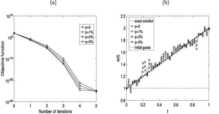
- (a) The objective function (10), and (b) the solutions for
, for
noise (Example 1).
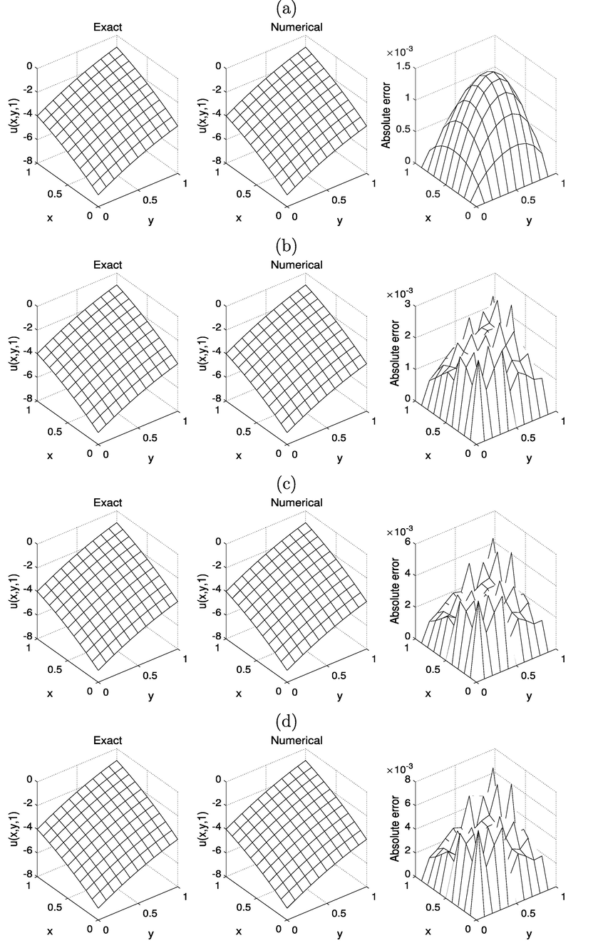
- The solutions for
, for: (a)
, (b)
, (c)
, and (d)
(Example 1).
We also take the source
. The previous example has reconstructed the smooth timewise thermal conductivity
given by (15). In this example, we assess the numerical reconstruction of a non-differentiable conductivity given by
We also have the same analytical solution for the temperature
given by (15). The initial guesses for the vector
for this example has been taken as
As in Example 1, for the numerical discretisation we employ the ADE with the mesh sizes
and
. Fig. 3(a) shows the rapidly decreasing functional (10) with the number of iterations. The results shown in Figs. 3(b) and 4, and in Table 2, yield the same conclusions as those obtained for Example 1.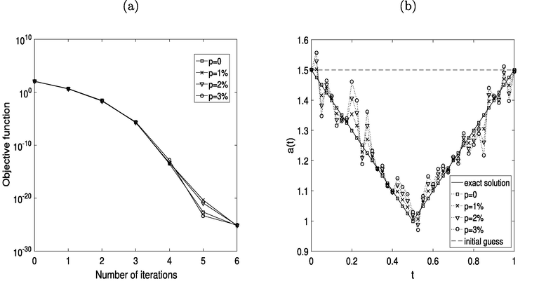
(a) The objective function (10), and (b) the solutions for
, for
noise (Example 2).
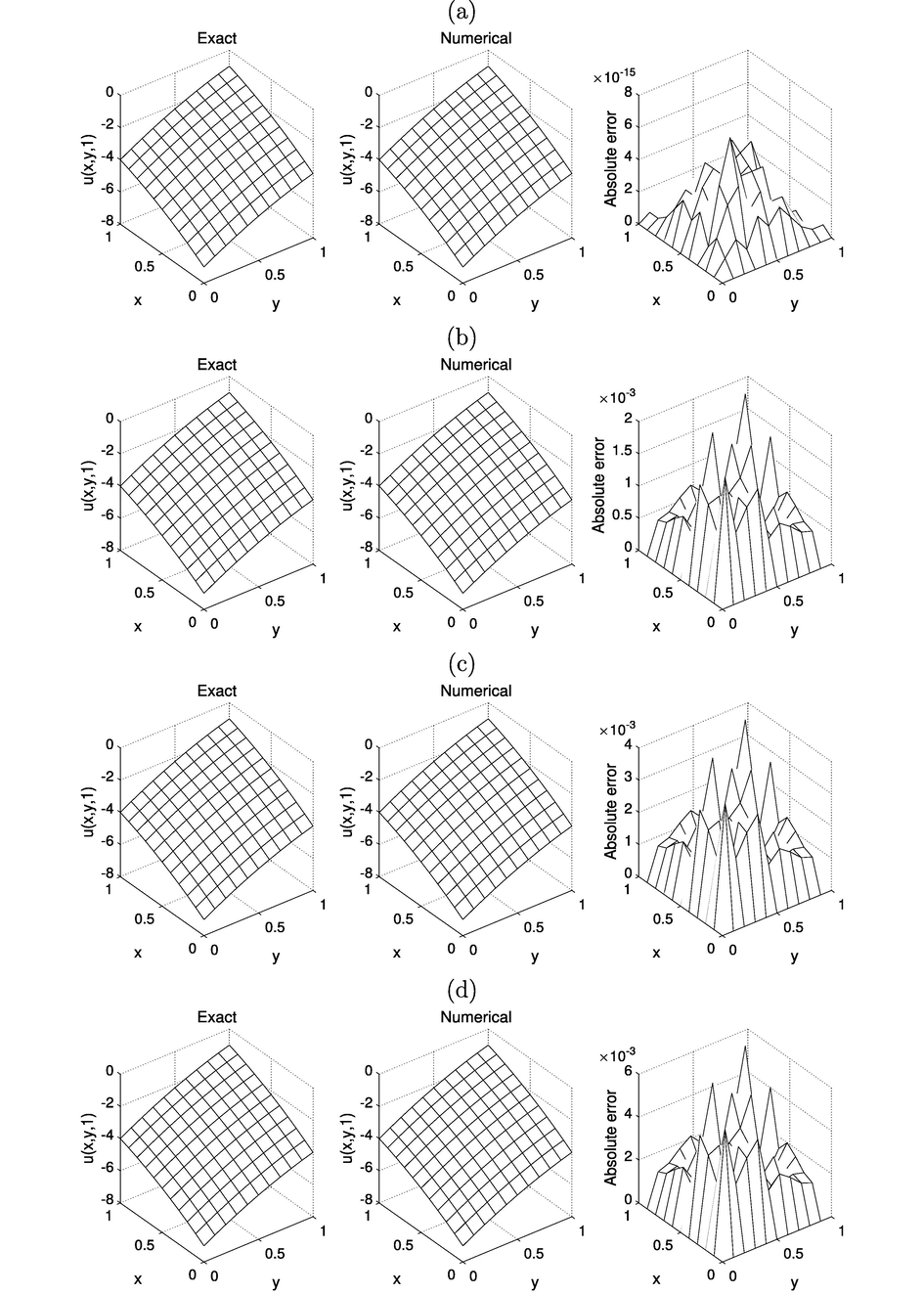
The solutions for
, for: (a)
, (b)
, (c)
, and (d)
noise (Example 2).
5 Conclusions
The reconstruction of conductivity and temperature from the non-local linear combination of heat flux over-determination (5) has been achieved numerically by employing the ADE, as a direct solver, implemented in a constrained minimization procedure. Further work will consist in retrieving multiple coefficients.
Declaration of interest
None.
References
- A box scheme for coupled systems resulting from microsensor thermistor problems. Dyn. Continuous Discrete Impulsive Syst.. 1999;5:209-223.
- [Google Scholar]
- On the solution of the diffusion equations by numerical methods. J. Heat Transfer. 1966;88:421-427.
- [Google Scholar]
- On the stability of alternating-direction explicit methods for advection-diffusion equations. Numer. Methods Partial Differ. Eqs.. 2007;23:1429-1444.
- [Google Scholar]
- The One-dimensional Heat Equation. Menlo Park, California: Addison-Wesley; 1984.
- A numerical procedure for diffusion subject to the specification of mass. Int. J. Eng. Sci.. 1993;31:347-355.
- [Google Scholar]
- A class of nonlinear nonclassical parabolic equations. J. Differ. Eqs.. 1989;79:266-288.
- [Google Scholar]
- An implicit finite difference scheme for the diffusion equation subject to mass specification. Int. J. Eng. Sci.. 1990;28:573-578.
- [Google Scholar]
- The significance of heterogeneity of evolving scales to transport in porous formations. Water Resour. Res.. 1994;13:33273-33336.
- [Google Scholar]
- Determination of Unknown Coefficients in the Heat Equation. University of Leeds; 2018. (Ph.D. thesis)
- An inverse problem of finding the time-dependent thermal conductivity from boundary data. Int. Commun. Heat Mass Transfer. 2017;301:147-154.
- [Google Scholar]
- An inverse problem of finding the time-dependent diffusion coefficient from an integral condition. Math. Methods Appl. Sci.. 2016;396:546-554.
- [Google Scholar]
- Inverse problem of determination of the leading coefficient of a two-dimensional parabolic equation. Matematychni Metody ta Fiziko-Mekhanichni Polya. 2004;47:7-16.
- [Google Scholar]
- A nonlocal inverse problem for the two-dimensional heat-conduction equation. J. Math. Sci.. 2018;231:558-571.
- [Google Scholar]
- Finite Difference Methods in Heat Transfer. Boca Raton, FL: CRC Press; 1994.
- Mathematical problems in viscoelasticity.Pitman Monographs and Surveys in Pure and Applied Mathematics. Vol vol. 35. Harlow: Longman Scientific & Technical; 1987.
- A nonlocal in time model for radionuclide propagation in Stokes fluid. Dinamika Sploshn. Sredy. 1993;107:180-193.
- [Google Scholar]


