RBF collocation approach to calculate numerically the solution of the nonlinear system of qFDEs

Fahimeh Akhavan Ghassabzadeh; Emran Tohidi; Harendra Singh; Stanford Shateyi

doi:10.1016/j.jksus.2020.101288

View/Download PDF

Buy Reprints

PDF

Translate this page into:

Original article

03 2020

:33;

101288

doi:

10.1016/j.jksus.2020.101288

RBF collocation approach to calculate numerically the solution of the nonlinear system of qFDEs

Fahimeh Akhavan Ghassabzadeh^{^a}, Emran Tohidi^{^b}, Harendra Singh^{^c}, Stanford Shateyi^{^d,⁎}

a Department of Mathematics, Faculty of Sciences, University of Gonabad, Gonabad, Iran

b Department of Mathematics, Kosar University of Bojnord, Bojnord P.O. Box 9415615458, Iran

c Department of Mathematics, Post-Graduate College, Ghazipur, 233001 Uttar Pradesh, India

d Department of Mathematics and Applied Mathematics, University of Venda, P. Bag X5050, Thohoyandu 0950, South Africa

⁎Corresponding author. stanford.shateyi@univen.ac.za (Stanford Shateyi)

Received: 2020-8-2, Accepted: 2020-11-23,

Disclaimer:
This article was originally published by Elsevier and was migrated to Scientific Scholar after the change of Publisher.

Peer review under responsibility of King Saud University.

Abstract

In this paper, we have implemented an efficient and high accurate radial basis function (RBF) collocation scheme for solving nonlinear systems of q-fractional differential equations. We firstly convert the problems under investigation into the equivalent systems of weakly singular q-integral equations by some essential results of fractional q-calculus. Secondly, we combine RBF collocation method and Newton–Raphson iterative algorithm to solve the latter systems of weakly singular q-integral equations. More precisely, applying RBF collocation scheme will transform the system of q-integral equations into the associated system of nonlinear algebraic equations that can be solved by iterative methods such as the Newton–Raphson algorithm. Finally, various numerical test problems including linear and nonlinear examples are listed to illustrate the robustness of the proposed global scheme with respect to the at least two recent methods in the literature.

Keywords

q-Fractional derivative

q-Fractional integral

q-Fractional differential equation

Radial basis functions

Collocation method

05A30

39A13

74H20

1 Introduction

Researchers in the field of mathematical modelling have investigated models and problems in different branches of science and engineering through the notion of fractional operators deeply (for instance, see Kilbas et al. (2006) and the references therein). This is because of the specific conditions of fractional operators, such as fractional integrals and derivatives of Riemann–Liouville and Caputo types. However, validating with experimental data and also parameter estimation in fractional calculus need to patience and hard attempts since, in fractional calculus, the domain of parameters is very wide to integer-order calculus.In addition to the classical Caputo and Riemann–Liouville types, fractional operators, several other new definitions such as Caputo and Fabrizio (2015) and Atangana and Baleanu (2016) fractional derivatives have been proposed by researchers in recent years for modelling different kinds of phenomena in engineering and science. However, some criticisms are presented for these new fractional derivatives and conclude that because of nonsigularity (in other words, countinuity) of the kernels of such these new tools, their applications for modelling in real-world are limited (Stynes, 2018). Therefore, nowadays two classical Caputo and Riemann–Liouville fractional derivatives are more popular and well-known between researchers and mathematicians.

In recent years, q-fractional calculus (as a particularl case of fractional calculus) was very popular among researchers. The definitions of q-fractional calculus originated from q-calculus (including q-integrals and q-derivatives) in classic calculus research works such as Jackson (1908) and Agarwal (1969). Caputo type q-fractional derivative is one of the most important definitions in this regard and has many applications in stochastic computations (Annaby and Mansour, 2012) and the mechanics of quantum (Kac and Cheung, 2002). As another typical example in the direction of applications of q-fractional derivatives, one can point out to the research work (Abdeljawad and Alzabut, 2018) that investigated the retarded logistic model. About recent studies about q-fractional differential equations, one can refer to the research articles that deal with the existence and uniqueness of the solutions and analytical methods. In Zhang and Guo (2020), the authors proved the existence and uniqueness of solutions of Catupo type q-fractional differential equations (with initial conditions) by using the q-analogy Gronwall inequality. Also, some investigations are made in the solution’s existence of some classes of boundary value problems (BVPs) in Almeida and Martins (2014). Stability analysis of some classes of q-fractional initial value problems (IVPs) was examined in detail via a Lyapunov approach (Jarad et al., 2013). Moreover, Tang and Zhang (2019) have some discussions regarding the analytical method of q-fractional differential equations by implementing the q-beta functions. Applications of Mittag–Leffler functions (in its q-analogy) for presenting some sets of solutions were conveyed in Abdeljawad and Baleanu (2011), Abdeljawad et al. (2012). After that, Salahshour et al. (2015) have been studied the rigorous convergence of the method proposed in Abdeljawad and Baleanu (2011). Variational iteration method (VIM) is also generalized to solve difference equations of q-fractional types by Wu and Baleanu (2013).

Despite extensive studies of q-fractional differential equations (qFDEs) by means of analytical methods, some very few research works were carried out to treat these types of equations numerically. Among the numerical approaches that are suggested and proposed to solve the Catupo type qFDEs, one can point out to Zhang and Tang (2019) as the first suggested local finite difference method (FDM). After that, as the second FDM in Lyu and Vong (2019), the authors proposed a second order convergent method with a full convergence analysis discussions in details. It should be noted, in Zhang and Tang (2019) just error of approximation is considered and convergence analysis was missed. As far as we know, fractional differential equations (FDEs) and specially qFDEs contain global fractional operators and solving them with local numerical techniques, such as FDM, will reduce the accuracy for computing the solutions. Therefore, researchers should provide some efficient global methods for calculating the solution with a high order of accuracy. This motivates us to investigate a very popular global numerical scheme in this regard. In this research work, we have considered a robust global numerical approach, radial basis function (RBF) collocation technique, for solving the following Caputo type qFDEs:

Problem (i) General form: The $α$ -order ( $0 < α < 1$ ) q-Caputo fractional order system

(1)

^{c} D_{q}^{α} y_{i} (t) = f_{i} (t, y_{1}, \dots, y_{n}), t_{0} < t ⩽ 1, i = 1, 2, \dots, n,

together with the initial conditions of the form

(2)

D_{q}^{j} y_{i} (t_{0}) = b_{ij}, (b_{ij} \in R i = 1, \dots, n; j = 0, 1, \dots, ⌈ α ⌉ - 1) .

Problem (ii) Special case of previous problem: The IVP of $α$ -order ( $0 < α < 1$ ) Caputo type q-fractional equation

(3)

^{c} D_{q}^{α} y (t) = f (t, y (t)), t_{0} < t ⩽ 1,

together with initial conditions

(4)

D_{q}^{j} y (t_{0}) = b_{j}, (b_{j} \in R j = 0, 1, \dots, ⌈ α ⌉ - 1),

where

t_{0} \in T_{q}, 0 < q < 1

and f is continuous. In this research work, we will study the approximate solutions of test problems

(i)

and

(ii)

by RBF collocation approach. This type of global schemes are very popular and well-known among the researchers in computational mathematics and have been applied for solving an extensive set of problems, see for instance Wei et al. (2018) and Wang and Wang (2016) and the references therein. Under some mild conditions, RBF collocation techniques have an exponential rate of accuracy. Taking into account that their precision is high and by applying a short number of localization points, they achieve to spectral accuracy as fast as possible. Since the application of these methods has had no results for solving Caputo type system of nonlinear qFDEs, this motivates us to investigate such these numerical approaches for solving them. This remnant of this research work formed as follows. Some primary notions and definitions of q-calculus and fractional derivatives are provided in Section 2. Sections 3 is devoted to the transformation of the basic Problems

(i)

and

(ii)

to the equivalent nonlinear weakly singular integral equations in the q-analogy form. Section 4 contains the implementation of RBF collocation approach for solving the equivalent nonlinear integral equations in the q-analogy form. Section 5 is designed to examine the proposed numerical approach for extensive test problems. In this Section, the accuracy of the proposed numerical technique is investigated in details experimentally by making some comparisons with respect to two recent local FDM schemes and superior numerical results show the robustness of our suggested global technique. Conclusions about the proposed method and also the plans for our future research works are given in Section 6.

2 Preliminary remarks

2.1

2.1 Essential results about q-calculus, fractional q-derivatives and q-integrals

Definition 1

(Zhang and Tang, 2019) The q-analogy of ${(t - x)}^{(γ)}$ is defined by

(5)

{(t - x)}^{(γ)} = t^{γ} Π_{i = 0}^{\infty} \frac{t - q^{i} x}{t - q^{γ + i} x} .

Definition 2

(Jackson, 1908) Let $g (t)$ be a real valued function on q-geometry set A and $∣ q ∣ < 1$ . The q-integral of $g (t)$ on interval $(a, b)$ is defined by

(6)

\int_{a}^{b} g (t) d_{q} t = \int_{0}^{b} g (t) d_{q} t - \int_{0}^{a} g (t) d_{q} t, a, b \in A,

where

(7)

\int_{0}^{x} g (t) d_{q} t = (1 - q) \sum_{n = 0}^{\infty} {xq}^{n} g ({xq}^{n}), x \in A .

Special cases include $\int_{0}^{1} {td}_{q} t = \frac{1}{1 + q},$ $\int_{0}^{1} t^{2} d_{q} t = \frac{1}{1 + q + q^{2}},$ $\int_{0}^{1} t^{n} d_{q} t = \frac{q - 1}{q^{n + 1} - 1} .$

Definition 3

(Jackson, 1908) Let $g (t)$ be a real valued function on q-geometry set A and $∣ q ∣ < 1$ . The q-derivative of $g (t)$ is defined by

(8)

D_{q} g (t) = \frac{g (qt) - g (t)}{(q - 1) t}, t \neq 0,

and

D_{q} g (t) = \lim_{n \to \infty} \frac{g ({tq}^{n}) - g (0)}{{tq}^{n}}, ∣ q ∣ < 1 .

Definition 4

(Atici and Eloe, 2007) For $0 < ∣ q ∣ < 1$ , the q-gamma function is defined By

(9)

Γ_{q} (α) = \frac{Π_{i = 0}^{K_{1}} (1 - q^{i + 1})}{Π_{i = 0}^{K_{2}} (1 - q^{i + α})} {(1 - q)}^{1 - α},

where

α \in C ⧹ {- n : n \in N^{*}}, 0 < | q | < 1

, and

K_{1}, K_{2} ⟶ \infty

Definition 5

(Atici and Eloe, 2007) Let $α ⩾ 0$ , the $α$ -order fractional q-integral of the Riemann–Liouville type is $(I_{q}^{0} g) (x) = g (x)$ and

(10)

(I_{q, a}^{α} g) (x) = \frac{1}{Γ (α)} \int_{a}^{x} {(x - qt)}^{(α - 1)} g (t) d_{q} t,

Definition 6

(Abdeljawad and Baleanu, 2011) The $α$ -order version of Caputo q-fractional derivative of a function $g (x) : (a, \infty) ⟶ R$ is defined by

(11)

(^{c} D_{q, a}^{α} g) (x) = \{\begin{matrix} (I_{q, a}^{- α} g) (x), α ⩽ 0 \\ (I_{q, a}^{⌈ α ⌉ - α} D_{q}^{⌈ α ⌉} g) (x), α > 0 . \end{matrix}

2.2

2.2 Radial basis functions collocation method

Given data at nodes $t_{0}, t_{1}, \dots, t_{n}$ in d dimension, the basic form for RBF interpolating is $S (t) = \sum_{j = 0}^{n} λ_{j} ϕ (| | t - t_{j} | |),$ where $| | \cdot | |$ denotes the Euclidean norm, $λ_{j}$ are the set of unknown coefficients to be determined. For scalar function values $g_{i} = g (t_{i})$ , the coefficients $λ_{j}$ are obtained by solving the following system of equations $[A] [\begin{matrix} λ_{0} \\ ⋮ \\ λ_{n} \end{matrix}] = [\begin{matrix} g_{0} \\ ⋮ \\ g_{n} \end{matrix}]$ where the interpolation matrix A satisfies $a_{ij} = ϕ (| | t_{i} - t_{j} | |)$ .

Some common types of RBF: Commonly used types of RBFs include the following forms in which $r = | | t - t_{i} | |$ and $∊$ is the shape parameter.

$•$ $ϕ_{∊} (r) = \sqrt{1 + {(∊ r)}^{2}}$ Multiquadrics(MQ).

$•$ $ϕ_{∊} (r) = e^{- {(∊ r)}^{2}}$ Gaussian.

$•$ $ϕ (r) = r^{3}$ Cubic.

$•$ $ϕ (r) = r^{2} Lnr$ Thin plate splines (TPS).

In this paper we focus on the popular choice of multiquadrics.

Instantly, we briefly introduce the RBFs collocation method. Consider the following boundary value problem when $Ω \subset R^{d}$ :

(12)

Lu = f in Ω

(13)

u = g on \partial Ω

where L is a linear differential operator. We distinguish in our notation center

X = \{x_{1}, \dots, x_{N}\}

and the collocation points

E = \{α_{1}, \dots, α_{N}\}

. Then we have the approximate solution of (12)–(13) in the form:

(14)

\tilde{u} (x) = \sum_{i = 1}^{N} λ_{i} ϕ (∥ x - x_{i} ∥),

where

λ_{i}, i = 1, 2, \dots, N

, are unknown coefficients that determined by collocation,

ϕ

is a RBF,

∥ . ∥

is the Euclidean norm and

x_{i}

is the center of the RBF.

Now, let $E$ divided into two subsets. One subset contains $N_{I}$ centers, $E_{1}$ , where Eq.(12) is enforced and the other subset contains $N_{B}$ centers, $E_{2}$ , where boundary conditions are enforced. So the collocation matrix has the following form: $M = [\begin{matrix} M_{I} \\ M_{B} \end{matrix}],$ in which, $M_{I} = L ϕ {(∥ α - x_{j} ∥)}_{α = α_{i}}, α_{i} \in E_{1}, x_{j} \in X$ , and $M_{B} = L ϕ {(∥ α - x_{j} ∥)}_{α = α_{i}}, α_{i} \in E_{2}, x_{j} \in X$ . The unknown coefficients $λ_{i}$ are determined by solving the linear system $M λ = F$ , where F is a vector included $f (α_{i}), α_{i} \in E_{1}$ , and $g (α_{i}), α_{i} \in E_{2}$ .

3 Discussion on equivalent problem

In this section, we deal with the equivalent form of the q-fractional models (1)–(2) and (3)–(4). For convenience, we need a Lemma for providing the proof of the main Theorem.

Lemma 1

Let $α > 0$ . If there exists $γ ⩽ α - ⌈ α ⌉ + 1$ such that $f \in C_{γ} [0, b]$ , then $I_{q}^{α} f \in C_{q}^{⌈ α ⌉} [0, b]$ .

Proof

See Annaby and Mansour (2012).

Theorem 1

Let $α > 0$ and $G_{i}$ be an open set in $C$ for $i = 1, \dots, n$ . Let $f_{i} (t, y_{1}, \dots, y_{n})$ be a function defined for $t \in (0, 1]$ , and $y_{i}$ in the domain $G_{i}$ , such that $f_{i} (t, y_{1}, \dots, y_{n}) \in C_{γ} [0, 1], γ ⩽ α - ⌈ α ⌉ + 1$ . If $y_{i} \in C_{q}^{⌈ α ⌉} [0, 1]$ then $y_{i}$ $(i = 1, \dots, n)$ satisfy (1)–(2) for all $t \in [0, 1]$ if only if $y_{i} (t)$ satisfies the q-integral system

(15)

y_{i} (t) = \sum_{j = 0}^{⌈ α ⌉ - 1} \frac{b_{ij}}{Γ_{q} (j + 1)} t^{j} + \frac{1}{Γ_{q} (α)} \int_{0}^{t} {(t - qs)}^{(α - 1)} f_{i} (s, y_{1} (s), \dots, y_{n} (s)) d_{q} s

for

i = 1, \dots, n

and all

t \in [0, 1]

Proof

Let $y_{i} (t)$ satisfy (1)–(2), then $^{c} D_{q}^{α} y_{i} (t) \in C_{γ} [0, 1]$ . Hence,

(16)

I_{q}^{α} (^{c} D_{q}^{α} y_{i} (t)) = y_{i} (t) - \sum_{j = 0}^{⌈ α ⌉ - 1} \frac{b_{ij}}{Γ_{q} (j + 1)} t^{j}, (0 ⩽ t ⩽ 1) .

On the other hand,

(17)

I_{q}^{α} (^{c} D_{q}^{α} y_{i} (t)) = I_{q}^{α} f_{i} (t, y_{1}, \dots, y_{n}) = \frac{1}{Γ_{q} (α)} \int_{0}^{t} {(t - qs)}^{(α - 1)} f (s, y_{1} (s), \dots, y_{n} (s)) d_{q} s

for all

t \in [0, 1]

. With combining (16) and (17) the necessity condition is proved. Now we prove the sufficiency condition. Let

y_{i} (t)

satisfies (15) for all

t \in [0, 1]

, then from Lemma 1,

y_{i} (t) \in C_{q}^{⌈ α ⌉} [0, 1]

. Consequently, acting on the two sides of (15) by the operator

_{c} D_{q}^{α}

we have

(18)

^{c} D_{q}^{α} y_{i} (t) = D_{q}^{α} [y_{i} (t) - \sum_{j = 0}^{⌈ α ⌉ - 1} \frac{b_{ij}}{Γ_{q} (j + 1)} t^{j}] = D_{q}^{α} I_{q}^{α} f_{i} (t, y_{1} (t), \dots, y_{n} (t)) = f_{i} (t, y_{1} (t), \dots, y_{n} (t)),

for all

t \in [0, 1]

. For

t \in (0, 1]

and

j \in \{0, 1, \dots, ⌈ α ⌉ - 1\}

, we get

(19)

D_{q}^{j} y_{i} (0^{+}) = \lim_{j \to \infty} D_{q}^{k} y_{i} ({tq}^{j}) = b_{ij} + \lim_{j \to \infty} I_{q}^{α - j} f_{i} ({tq}^{j}, y_{1} ({tq}^{j}), \dots, y_{n} ({tq}^{j})) = b_{ij} + \lim_{j \to \infty} \frac{1}{Γ_{q} (α - j)} \int_{0}^{{tq}^{j}} {(t - qs)}^{(α - 1 - j)} f_{i} (s, y_{1} (s), \dots, y_{n} (s)) d_{q} s = b_{ij} + \lim_{j \to \infty} \frac{1}{Γ_{q} (α - j)} \sum_{r = j}^{\infty} q^{r} \frac{{(q^{α - j}; q)}_{r}}{{(q; q)}_{r}} f_{i} ({tq}^{j}, y_{1} ({tq}^{j}), \dots, y_{n} ({tq}^{j})),

where the limit on the most rigth hand side of (19) vanishes because of

f_{i} (t, y_{1} (t), \dots, y_{n} (t)) \in C_{γ} [0, 1]

Therefore, every solution of The q-Caputo fractional order system (1)–(2) is also a solution of the q-Volterra integral system (15) and vice versa.

Similarly, one can show that the initial value problem of $α_{-}$ order Caputo type q-fractional Eqs. (3)–(4) is equivalent with the following q-integral equation:

(20)

y (t) = \sum_{j = 0}^{⌈ α ⌉ - 1} \frac{b_{j}}{Γ_{q} (j + 1)} t^{j} + \frac{t^{α - 1}}{Γ_{q} (α)} \int_{0}^{t} {(t - qs)}^{(α - 1)} f (s, y (s)) d_{q} s .

So, every solution of q-fractional initial value problem (3)–(4) is also a solution of the q-Volterra integral Eq.(20)vice versa.

4 Outline of the approximation method

In this section, an algorithm for the approximate solution of the two q-fractional models (1)–(2) and (3)–(4) will be derived. We assume that $0 = t_{0} < t_{1} < \dots < t_{N} = 1$ be a nonuniform mesh on $[0, 1]$ with $t_{i} = q^{N - i} \in T_{q}$ , for $i = 0, 1, \dots, N$ .

problem (i): (see Eqs. (1), (2)) In this case by using Definition 2 and Eq. (15), for $i = 1, \dots, n$ , we get

(21)

y_{i} (t) = \sum_{j = 0}^{⌈ α ⌉ - 1} \frac{b_{ij}}{Γ_{q} (j + 1)} t^{j} + \frac{(1 - q)}{Γ_{q} (α)} \sum_{k = 0}^{\infty} {tq}^{k} {(t - {tq}^{(k + 1)})}^{(α - 1)} f_{i} ({tq}^{k}, y_{1} ({tq}^{k}), \dots, y_{n} ({tq}^{k})) d_{q} s .

Collocating Eq. (21) at the nodes $t_{l}$ yeilds

(22)

y_{i} (t_{l}) = \sum_{j = 0}^{⌈ α ⌉ - 1} \frac{b_{ij}}{Γ_{q} (j + 1)} t_{l}^{j} + \frac{(1 - q)}{Γ_{q} (α)} \sum_{k = 0}^{\infty} t_{l} q^{k} {(t_{l} - t_{l} q^{(k + 1)})}^{(α - 1)} f_{i} (t_{l} q^{k}, y_{1} (t_{l} q^{k}), \dots, y_{n} (t_{l} q^{k})) d_{q} s .

We suppose that $M_{1}$ be a positive integer, $y_{il} = y_{i} (t_{l})$ and

(23)

y_{i} (t) \approx y_{i}^{N} (t) = \sum_{ρ = 0}^{N} λ_{i ρ} φ_{ρ} (t),

where

φ_{ρ} (t)

and

λ_{i ρ} (ρ = 0, 1, \dots, N; i = 1, \dots, n)

are the radial basis functions and unknown RBF coefficients, respectively. Since

y_{i}^{N} (t)

is the approximation of

y_{i} (t)

, we can write

(24)

y_{i}^{N} (t_{l}) \approx \sum_{j = 0}^{⌈ α ⌉ - 1} \frac{b_{ij}}{Γ_{q} (j + 1)} t_{l}^{j} + \frac{(1 - q)}{Γ_{q} (α)} \sum_{k = 0}^{M_{1}} t_{l} q^{k} {(t_{l} - t_{l} q^{(k + 1)})}^{(α - 1)} f_{i} (t_{l} q^{k}, y_{1}^{N} (t_{l} q^{k}), \dots, y_{n}^{N} (t_{l} q^{k})) d_{q} s .

So, we have a nonlinear algebraic system with $nN + n$ equations and $nN + n$ unknowns $λ_{i ρ} (ρ = 0, 1, \dots, N; i = 1, \dots, n)$ . The algebraic system (24) can be solved by any suitable direct or iterative method. In this paper, we will use fsolve command, which its default is the NewtonRaphson iterative algorithm, in MATLAB software.

problem (ii): (see Eqs. (3), (4)) In this case, we consider two following states:

(a) $f (t, y (t)) = \sum_{i = 1}^{n} μ_{i} t^{ϑ_{i}}$ with constant $μ_{i}$ and $ϑ_{i}$ .

Theorem 2

Let $f (t, y (t)) = \sum_{i = 1}^{n} μ_{i} t^{ϑ_{i}}$ with constant $μ_{i}$ and $ϑ_{i}$ . Then the solution of problem (3)–(4) is

(25)

y (t) = \sum_{j = 0}^{⌈ α ⌉ - 1} \frac{b_{j}}{Γ_{q} (j + 1)} t^{j} + \frac{t^{α} (1 - q)}{Γ_{q} (α)} \sum_{r = 0}^{\infty} q^{r} (Π_{k = 0}^{\infty} \frac{1 - q^{r + k + 1}}{1 - q^{r + α + i}}) \sum_{i = 1}^{n} μ_{i} {({tq}^{r})}^{ϑ_{i}} .

Proof

We know that problem (3)–(4) is equivalent to Eq. (20), on the other hand, from Definition 2, we get

(26)

\int_{0}^{t} {(t - qs)}^{(α - 1)} f (s, y (s)) d_{q} s = (1 - q) \sum_{r = 0}^{\infty} {tq}^{r} {(t - {tq}^{r + 1})}^{(α - 1)} \sum_{i = 1}^{n} μ_{i} {({tq}^{r})}^{ϑ_{i}} .

Using Definition 1 implies that

(27)

y (t) = \sum_{j = 0}^{⌈ α ⌉ - 1} \frac{b_{j}}{Γ_{q} (j + 1)} t^{j} + \frac{t^{α} (1 - q)}{Γ_{q} (α)} \sum_{r = 0}^{\infty} q^{r} (Π_{k = 0}^{\infty} \frac{1 - q^{r + k + 1}}{1 - q^{r + α + i}}) \sum_{i = 1}^{n} μ_{i} {({tq}^{r})}^{ϑ_{i}} .

Let $M_{2}$ and $M_{3}$ be two positive integers, so, in this case $y (t)$ can be easily estimated with the following

(28)

y (t) \approx \sum_{j = 0}^{⌈ α ⌉ - 1} \frac{b_{j}}{Γ_{q} (j + 1)} t^{j} + \frac{t^{α} (1 - q)}{Γ_{q} (α)} \sum_{r = 0}^{M_{2}} q^{r} (Π_{k = 0}^{M_{3}} \frac{1 - q^{r + k + 1}}{1 - q^{r + α + i}}) \sum_{i = 1}^{n} μ_{i} {({tq}^{r})}^{ϑ_{i}} .

(b) $f (t, y (t)) = g (t) + h (t) F (y (t))$ where $h (t) ≅ 0$ .

In this case, by substituting (5) and (7) in Eq. (20), we obtain

(29)

y (t) = \sum_{j = 0}^{⌈ α ⌉ - 1} \frac{b_{j}}{Γ_{q} (j + 1)} t^{j} + \frac{t^{α} (1 - q)}{Γ_{q} (α)} \sum_{r = 0}^{\infty} q^{r} (Π_{k = 0}^{\infty} \frac{1 - q^{r + k + 1}}{1 - q^{r + α + i}}) (g ({tq}^{r}) + h ({tq}^{r}) F (y ({tq}^{r}))) .

After collocate Eq. (29) at $N + 1$ points $t_{i}$ , for $i = 0, 1, \dots, N$ , we have

(30)

y (t_{i}) = \sum_{j = 0}^{⌈ α ⌉ - 1} \frac{b_{j}}{Γ_{q} (j + 1)} t_{i}^{j} + \frac{t^{α} (1 - q)}{Γ_{q} (α)} \sum_{r = 0}^{\infty} q^{r} (Π_{k = 0}^{\infty} \frac{1 - q^{r + k + 1}}{1 - q^{r + α + i}}) (g (t_{i} q^{r}) + h (t_{i} q^{r}) F (y (t_{i} q^{r}))) .

Now, let $M_{2}$ and $M_{3}$ be positive integers, $y_{i} = y (t_{i})$ and

(31)

y (t) \approx y^{N} (t) = \sum_{j = 0}^{N} λ_{j} φ_{j} (t),

where

φ_{j} (t)

and

λ_{j} (j = 0, 1, \dots, N)

are the radial basis functions and unknown RBF coefficients, respectively. So, we obtain the following system of nonlinear algebric equation

(32)

\sum_{j = 0}^{N} λ_{j} φ_{j} (t_{i}) \approx \sum_{j = 0}^{⌈ α ⌉ - 1} \frac{b_{j}}{Γ_{q} (j + 1)} t_{i}^{j} + \frac{t_{i}^{α} (1 - q)}{Γ_{q} (α)} \sum_{r = 0}^{M_{2}} q^{r} (Π_{k = 0}^{M_{3}} \frac{1 - q^{r + k + 1}}{1 - q^{r + α + i}}) (g (t_{i} q^{r}) + h (t_{i} q^{r}) F (\sum_{j = 0}^{N} λ_{j} φ_{j} (t_{i} q^{r}))) .

with

N + 1

unknowns

λ_{j} (j = 0, 1, \dots, N)

. We will use fsolve Matlab’s command for solving this system.

5 Examination of the method experimentally

To show the efficiency and accuracy of the earlier described method, we present in this section some significant examples.All of the programs associated with the implementation of the suggested method for solving the studied examples are written in MATLAB 2016b in a Laptop PC with 4 GB Ram. It should be noted that the default MATLAB’s tolerance is used in the fsolve solver. We set $M_{1} = M_{2} = M_{3} = K_{1} = K_{2} = 100$ in all computations. The Multiquadric radial basis function is used in the approximated solutions (24) and (31), and the trial and error method is applied for choosing shape parameters.

Example 1

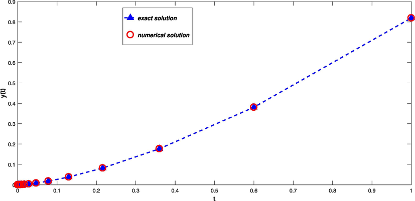
First, we consider the following Caputo type q-fractional initial value problem $\begin{matrix} ^{c} D_{q}^{\frac{1}{2}} y (t) = t, 0 < t \leq 1, \\ y (0) = 0 . \end{matrix}$

The exact solution is $y (t) = \frac{Γ_{q} (2)}{Γ_{q} (\frac{5}{2})} t^{\frac{3}{2}}$ . The exact and approximated solution at $N = 10$ , are shown in Fig. 1.The obtained results for Example 1 are compared the results in Zhang and Tang (2019), in Table 1. From this table, one can see high accuracy of the proposed method.

Example 2

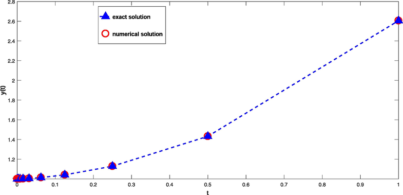
Consider the Caputo type q-fractional initial value problem $\begin{matrix} ^{c} D_{q}^{\frac{1}{2}} y (t) = t + t^{2}, 0 < t \leq 1, \\ y (0) = 1 . \end{matrix}$

The exact solution is $y (t) = 1 + \frac{Γ_{q} (2)}{Γ_{q} (\frac{5}{2})} t^{\frac{3}{2}} + \frac{Γ_{q} (3)}{Γ_{q} (\frac{7}{2})} t^{\frac{5}{2}}$ .Fig. 2 shows the exact solution and approximated solution at N = 10. Absolute value error is reported in Table 2. It is obvious from these Figure and Table that, the suggested scheme is very accurate.

Example 3

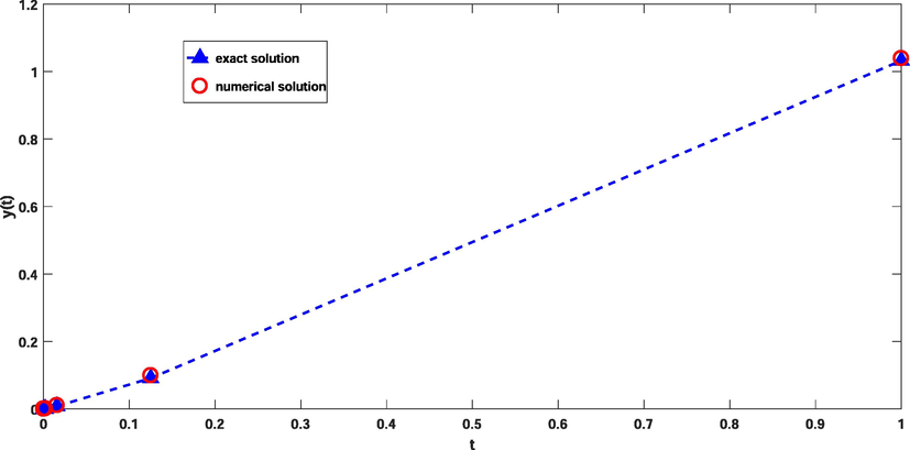
Consider the following nonlinear Caputo type q-fractional initial value problem $\begin{matrix} ^{c} D_{q}^{\frac{1}{3}} y (t) = t^{\frac{- 3}{2}} y^{2} (t), 0 < t \leq 1, \\ y (0) = 0.0001 . \end{matrix}$

The exact solution of this problem is $y (t) = 0.0001 + \frac{Γ_{q} (\frac{13}{6})}{Γ_{q} (\frac{11}{6})} t^{\frac{7}{6}}$ . The numerical results, for $N = 10, q = \frac{1}{8}$ and $α = \frac{1}{3}$ , are presented in Fig. 3 and Table 3. A simple comparison between of the proposed scheme and the numerical results of Thang and Zhang (2019) (i.e., iterative scheme) confirms the accuracy of our proposed method.

Example 4

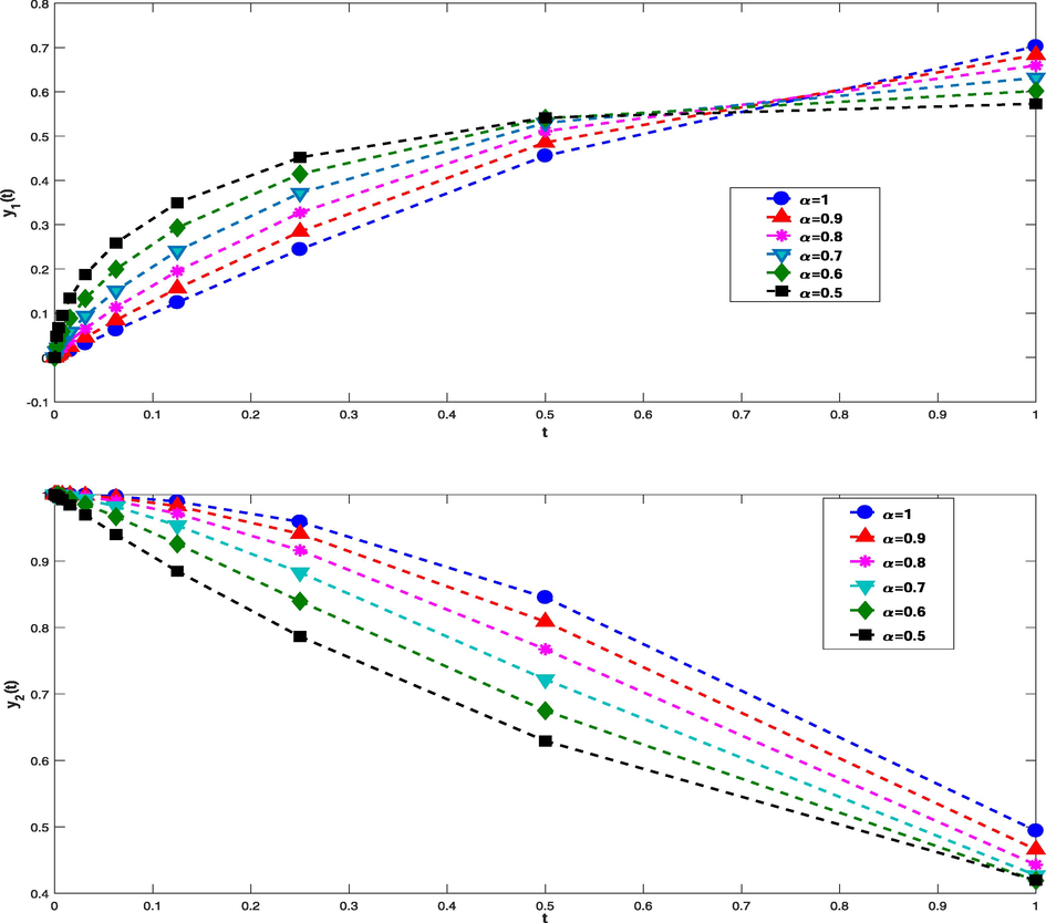
Consider the q-Caputo fractional order system $\begin{matrix} ^{c} D_{q}^{α} y_{1} (t) = y_{2} (t),^{c} D_{q}^{α} y_{2} (t) = - y_{1} (t) 0 < t \leq 1, \\ y_{1} (0) = 0 y_{2} (0) = 1 . \end{matrix}$

The exact solution is $y_{1} (t) = t^{α} \sum_{j = 0}^{M} {(- 1)}^{j} \frac{t^{2 α j}}{Γ_{q} (2 α j + α + 1)}$ and $y_{2} (t) = \sum_{j = 0}^{M} {(- 1)}^{j} \frac{t^{2 α j}}{Γ_{q} (2 α j + 1)}$ , that $M ⟶ \infty$ . We set $M = 10$ in the reported exact solution in Tables 4 and 5. For $α = 1$ , we obtain $y_{1} (t) = \sin_{q} t (1 - q)$ and $y_{2} (t) = \cos_{q} t (1 - q)$ ( $| t (1 - q) | < 1$ ). In Fig. 4, we have plotted the approximated solutions behaviour for different values of fractional and integer- order derivatives. Also, in Tables 4 and 5 we illustrate the errors associated to the presented method. From this tables, one can see high accuracy of the proposed method.

Example 5

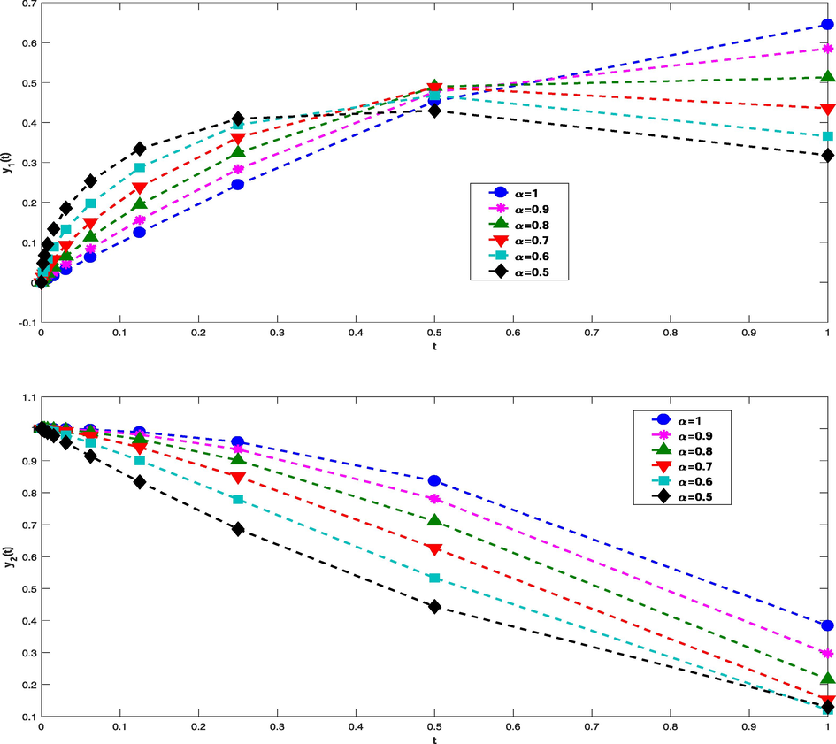
Consider the q-Caputo fractional order system $\begin{matrix} ^{c} D_{q}^{α} y_{1} (t) = y_{2} (t),^{c} D_{q}^{α} y_{2} (t) = - q^{- α} y_{1} (qt) 0 < t \leq 1, \\ y_{1} (0) = 0 y_{2} (0) = 1 . \end{matrix}$

The exact solution is $y_{1} (t) = t^{α} \sum_{j = 0}^{M} {(- 1)}^{j} q^{j (j - 1) α} \frac{t^{2 α j}}{Γ_{q} (2 α j + α + 1)}$ and $y_{2} (t) = \sum_{j = 0}^{M} {(- 1)}^{j} q^{j (j - 1) α} \frac{t^{2 α j}}{Γ_{q} (2 α j + 1)}$ , that $M ⟶ \infty$ . We set $M = 10$ in the reported exact solution in Tables 6 and 7.

In Fig. 5, we have plotted the approximated solutions behaviour for different values of fractional and integer-order derivatives. Also, in Tables 6 and 7 we illustrate the errors associated to the presented method. From this tables, one can see high accuracy of the proposed method.

Numerical solution and exact solution for Example 1 N = 20 , q = 3 / 5 , α = 1 / 2 ).

Table 1 Numerical solution and absolute value error for Example 1 (

N = 20, q = 3 / 5, α = 1 / 2

t	$y (t)$	$y^{N} (t)$	Absolute error	Method in Zhang and Tang (2019)
0	0	0	0	0
${(3 / 5)}^{1} 9$	$0.000000389570411$	$0.000000389570411$	$1.58819 e - 22$	$4.44849 e - 08$
${(3 / 5)}^{1} 7$	$0.000001803566719$	$0.000001803566719$	$8.47033 e - 22$	$2.29471 e - 08$
${(3 / 5)}^{1} 5$	$0.000008349845921$	$0.000008349845921$	$3.38813 e - 21$	$1.20204 e - 07$
${(3 / 5)}^{1} 3$	$0.000038656694080$	$0.000038656694080$	$1.35525 e - 20$	$5.72027 e - 08$
${(3 / 5)}^{1} 1$	$0.000178966176295$	$0.000178966176295$	$1.35525 e - 20$	$3.23198 e - 08$
${(3 / 5)}^{9}$	$0.000828547112477$	$0.000828547112477$	$3.25261 e - 19$	$1.90138 e - 08$
${(3 / 5)}^{7}$	$0.003835866261468$	$0.003835866261468$	$1.30104 e - 18$	$1.13302 e - 08$
${(3 / 5)}^{5}$	$0.017758640099387$	$0.017758640099387$	$6.93889 e - 18$	$6.78151 e - 09$
${(3 / 5)}^{3}$	$0.082215926386051$	$0.082215926386051$	$2.77556 e - 17$	$4.06534 e - 09$
$(3 / 5)$	$0.380629288824312$	$0.380629288824311$	$1.11022 e - 16$	$1.22486 e - 07$
1	$0.818983831497407$	$0.818983831497406$	$3.33067 e - 16$	$5.42886 e - 08$

Numerical solution and exact solution for Example 2 N = 10 , q = 1 / 2 , α = 1 / 2 ).

Table 2 Numerical solution and absolute value error for Example 2

N = 10, q = 1 / 2, α = 1 / 2

t	$Y (t)$	$Y^{N} (t)$	Absolute value error
0	$1.000000000000000$	$1.000000000000000$	0
${(1 / 2)}^{9}$	$1.000072627919360$	$1.000072627919360$	0
${(1 / 2)}^{8}$	$1.000205787657204$	$1.000205787657204$	0
${(1 / 2)}^{7}$	$1.000584119464960$	$1.000584119464960$	0
${(1 / 2)}^{6}$	$1.001663815501096$	$1.001663815501096$	0
${(1 / 2)}^{5}$	$1.004772031242264$	$1.004772031242264$	$2.22045 e - 16$
${(1 / 2)}^{4}$	$1.013870979799737$	$1.000828547112477$	$2.22045 e - 16$
${(1 / 2)}^{3}$	$1.041346666660917$	$1.041346666660917$	$2.22044 e - 16$
${(1 / 2)}^{2}$	$1.128902423708945$	$1.128902423708945$	0
$(1 / 2)$	$1.432226668417044$	$1.432226668417043$	$4.44089 e - 16$
1	$2.605126119625209$	$2.605126119625208$	$1.3323 e - 15$

Numerical solution and exact solution for Example 3 N = 10 , q = 1 / 8 , α = 1 / 3 ).

Table 3 Numerical solution and absolute value error for Example 3

N = 10, q = 1 / 8, α = 1 / 3

t	$y (t)$	$y^{N} (t)$	Absolute value error	Method in Tang and Zhang (2019)
0	$0.000100000000000$	$0.000100000000000$	0	0
${(1 / 8)}^{9}$	$0.000100000339875$	$0.000235644848742$	$1.35645 e - 04$	$7.10653 e - 04$
${(1 / 8)}^{8}$	$0.000100003845252$	$0.000235645502072$	$1.35642 e - 04$	$1.59919 e - 03$
${(1 / 8)}^{7}$	$0.000100043504059$	$0.000235650833029$	$1.35607 e - 04$	$3.59173 e - 03$
${(1 / 8)}^{6}$	$0.000100492192244$	$0.000235700154354$	$1.35208 e - 04$	$8.06390 e - 03$
${(1 / 8)}^{5}$	$0.000105568519578$	$0.000236520354251$	$1.30952 e - 04$	$1.81032 e - 02$
${(1 / 8)}^{4}$	$0.000163000607271$	$0.000268923723107$	$1.05923 e - 04$	$4.06404 e - 02$
${(1 / 8)}^{3}$	$0.000812770505922$	$0.001174594502890$	$3.61824 e - 03$	$9.12346 e - 02$
${(1 / 8)}^{2}$	$0.008164077730671$	$0.010408552873172$	$2.24448 e - 03$	$2.04815 e - 01$
$(1 / 8)$	$0.091334624757964$	$0.099095364598783$	$7.76074 e - 03$	$4.59794 e - 01$
1	$1.032301949525868$	$1.038672793906552$	$6.37084 e - 03$	$1.03220$

Table 4 Numerical solution and absolute error for Example 4

N = 10, q = 1 / 2, α = 1

t	$y_{1} (t)$	$y_{1}^{N} (t)$	Absolute error
0	0	$0.000000000001337$	$1.33683 e - 12$
${(1 / 2)}^{9}$	$0.001953122161687$	$0.001953122160983$	$7.03764 e - 13$
${(1 / 2)}^{8}$	$0.003906227293564$	$0.003906227290589$	$2.97537 e - 12$
${(1 / 2)}^{7}$	$0.007812318350801$	$0.007812318350060$	$7.41147 e - 13$
${(1 / 2)}^{6}$	$0.015623546879650$	$0.015623546876897$	$2.75346 e - 12$
${(1 / 2)}^{5}$	$0.031238377380371$	$0.031238377378862$	$1.50979 e - 12$
${(1 / 2)}^{4}$	$0.062407093954124$	$0.062407093947164$	$6.95929 e - 12$
${(1 / 2)}^{3}$	$0.124259139836641$	$0.124259139839404$	$2.76279 e - 12$
${(1 / 2)}^{2}$	$0.244148412653959$	$0.244148412650705$	$3.25428 e - 12$
$(1 / 2)$	$0.455460666624558$	$0.455460666640393$	$1.58348 e - 11$
1	$0.702468139652606$	$0.702468139646127$	$6.47926 e - 12$

Table 5 Numerical solution and absolute error for Example 4

N = 10, q = 1 / 2, α = 1

)

t	$y_{2} (t)$	$y_{2}^{N} (t)$	Absolute error
0	$1.000000000000000$	$0.999999999998487$	$1.51257 e - 12$
${(1 / 2)}^{9}$	$0.999997456871446$	$0.999997456864538$	$6.90803 e - 12$
${(1 / 2)}^{8}$	$0.999989827521264$	$0.999989827520871$	$3.930194 e - 13$
${(1 / 2)}^{7}$	$0.999959310652706$	$0.999959310658919$	$6.21358 e - 12$
${(1 / 2)}^{6}$	$0.999837251692708$	$0.999837251699265$	$6.55653 e - 12$
${(1 / 2)}^{5}$	$0.999349152046140$	$0.999349152053606$	$7.46603 e - 12$
${(1 / 2)}^{4}$	$0.997398930360074$	$0.997398930361860$	$1.78668 e - 12$
${(1 / 2)}^{3}$	$0.989632734120284$	$0.989632734133493$	$1.32099 e - 11$
${(1 / 2)}^{2}$	$0.959114182538539$	$0.959114182536891$	$1.64735 e - 12$
$(1 / 2)$	$0.845249015882399$	$0.845249015891874$	$9.47542 e - 12$
1	$0.494014946056096$	$0.494014946047678$	$8.41804 e - 12$

Numerical solution for different value of α for Example 4 N = 10 , q = 1 / 2 ).

Table 6 Numerical results for Example 5

N = 10, q = 1 / 3, α = 1

t	$y_{1} (t)$	$y_{1}^{N} (t)$	$\| y_{1} - y_{1}^{N} \|$
0	0	$8.399500539546523 e - 11$	$8.3995 e - 11$
${(1 / 3)}^{9}$	$5.080526335720037 e - 05$	$5.080527530022111 e - 05$	$1.1943 e - 11$
${(1 / 3)}^{8}$	$1.524157884374290 e - 04$	$1.524157231143283 e - 04$	$6.5323 e - 11$
${(1 / 3)}^{7}$	$4.572473211896416 e - 04$	$4.572472881195014 e - 04$	$3.3070 e - 11$
${(1 / 3)}^{6}$	$0.001371740772258$	$0.001371740956903$	$1.8465 e - 10$
${(1 / 3)}^{5}$	$0.004115190151394$	$0.004115190393954$	$2.4256 e - 10$
${(1 / 3)}^{4}$	$0.012344701995526$	$0.012344701915369$	$8.0156 e - 11$
${(1 / 3)}^{3}$	$0.037010659197795$	$0.037010658981692$	$2.1610 e - 10$
${(1 / 3)}^{2}$	$0.110399301846614$	$0.110399301891554$	$4.4940 e - 11$
$(1 / 3)$	$0.314209777667648$	$0.314209777829496$	$1.6185 e - 10$
1	$0.506694834907219$	$0.506694834174431$	$7.3279 e - 10$

Table 7 Numerical results for Example 5

N = 10, q = 1 / 3, α = 1

t	$y_{2} (t)$	$y_{2}^{N} (t)$	$\| y_{2} - y_{2}^{N} \|$
0	1	$0.999999999929966$	$7.0034 e - 11$
${(1 / 3)}^{9}$	$0.999999998064119$	$0.999999998048430$	$1.5689 e - 11$
${(1 / 3)}^{8}$	$0.999999982577070$	$0.999999982503621$	$7.3449 e - 11$
${(1 / 3)}^{7}$	$0.999999843193633$	$0.999999843202192$	$8.5587 e - 12$
${(1 / 3)}^{6}$	$0.999998588742821$	$0.999998588786891$	$4.4071 e - 11$
${(1 / 3)}^{5}$	$0.999987298695312$	$0.999987298717936$	$2.2623 e - 11$
${(1 / 3)}^{4}$	$0.999885689061944$	$0.999885689020719$	$4.1225 e - 11$
${(1 / 3)}^{3}$	$0.998971266691906$	$0.998971266679367$	$1.2539 e - 11$
${(1 / 3)}^{2}$	$0.990746675759062$	$0.990746675981385$	$2.2232 e - 10$
$(1 / 3)$	$0.917147141194653$	$0.917147141235329$	$4.0676 e - 11$
1	$0.288727585859356$	$0.288727585896525$	$3.7169 e - 11$

Numerical solution for different value of α for Example 5 N = 10 , q = 1 / 2 ).

6 Conclusions and future works

In this article, a high accurate global numerical framework (i.e., RBF collocation approach) has been proposed for solving system of nonlinear qFDEs of Caputo type. This type of problems was investigated by analytical methods extensively, but from the numerical point of view, only two recent research works (i.e. FDMs) were suggested to solve them approximately. As far as we know, this is the first paper that solve these equations numerically and globally. Applying a short number of collocation points give us accurate results as fast as possible. Superior numerical results with respect to two recent numerical schemes motive us to implement the method for solving other types of q-fractional models and test problems. As our future research work, we will investigate numerical treatment of q-version of time-fractional diffusion (Ghanbari and Atangana, 2020), Burgers (Akram et al., 2020), foam drainage (Al-Mdallal et al., 2020; Shi et al., 2020), coupled kaup-kupershmidt (Wang et al., 2019), Klein–Gordon (Akram et al., 2020), Shrodinger (Ain, YYYY), Telegraph (Akram et al., 2020), Levi (Feng, 2020) and Ginzburg–Landau equations (Al-Ghafri, 2020).

Declaration of Competing Interest

The authors declare that they have no known competing financial interests or personal relationships that could have appeared to influence the work reported in this paper.

References

Abdeljawad T., Benli B., Baleanu D., . A generalized q-Mittag-Leffler function by q-Caputo fractional linear equations. Abstr. Appl. Anal.. 2012;2012:1-11.
[Google Scholar]
Abdeljawad T., Baleanu D., . Caputo q-fractional initial value problems and a q-analogue Mittag-Leffler function. Commun. Nonlinear Sci. Numer. Simul.. 2011;16:4682-4688.
[Google Scholar]
Abdeljawad T., Alzabut J., . On Riemann-Liouville fractional q-difference equations and their application to retarded logistic type model. Math. Methods Appl. Sci.. 2018;41:8953-8962.
[Google Scholar]
Agarwal R.P., . Certain fractional q-integrals and q-derivatives. Proc. Camb. Phil. Soc.. 1969;66:365-370.
[Google Scholar]
Akram T., Abbas M., Iqbal A., Baleanu D., Asad J.H., . Novel numerical approach based on modified extended cubic B-spline functions for solving non-linear time-fractional telegraph equation. Symmetry. 2020;12:1154.
[Google Scholar]
Almeida R., Martins N., . Existence results for fractional q-difference equations of order α∈(2,3)) with three-point boundary conditions. Commun. Nonlinear Sci. Numer. Simul.. 2014;19:1675-1685.
[Google Scholar]
Akram T., Abbas M., Riaz M.B., Ismail A.I., Ali N.M., . Development and analysis of new approximation of extended cubic B-spline to the non-linear time fractional Klein-Gordon equation. Fractals. 2020;28:1-20.
[Google Scholar]
Akram T., Abbas M., Riaz M.B., Ismail A.I., Ali N.M., . An efficient numerical technique for solving time fractional Burgers equation. Alex. Eng. J.. 2020;59(4):2201-2220.
[CrossRef] [Google Scholar]
Al-Ghafri Kh.S., . Soliton behaviours for the conformable space-time fractional complex Ginzburg-Landau equation in optical fibers. Symmetry. 2020;12:1-14.
[Google Scholar]
Annaby M.H., Mansour Z.S., . q-Fractional Calculus and Equations. New York: Springer Heidelberg; 2012.
Atangana A., Baleanu D., . New fractional derivatives with non-local and non-singular kernel: theory and applications to heat transfer model. Therm. Sci.. 2016;20:763-769.
[Google Scholar]
Atici F.M., Eloe P.W., . Fractional q-calculus on a time scale. J. Nonlinear Math. Phys.. 2007;14:341-352.
[Google Scholar]
Caputo M., Fabrizio M., . A new definition of fractional derivative without singular kernel. Prog. Fract. Differ. Appl.. 2015;1:73-85.
[Google Scholar]
Feng W., . Exact solutions and conservation laws of time-fractional Levi equation. Symmetry. 2020;12:1-13.
[Google Scholar]
Ghanbari B., Atangana A., . An efficient numerical approach for fractional diffusion partial differential equations. Alex. Eng. J.. 2020;59:2171-2180.
[Google Scholar]
Jackson F.H., . On q-functions and a certain difference operator. Trans. R. Soc. Edinb.. 1908;46:64-72.
[Google Scholar]
Jarad F., Abdeljawad T., Baleanu D., . Stability of q-fractional non-autonomous systems. Nonlinear Anal. Real World Appl.. 2013;14:780-784.
[Google Scholar]
Kac V., Cheung P., . Quantum Calculus. New York: Springer-Verlag; 2002.
Kilbas A.A., Srivastava H.M., Trujillo J.J., . Theory and Applications of Fractional Differential Equations, NorthHolland Mathematics Studies. Vol 207. Amsterdam: Elsevier; 2006.
Al-Mdallal Q.M., Yusuf H., Ali A., . A novel algorithm for time-fractional foam drainage equation. Alex. Eng. J.. 2020;59:1607-1621.
[Google Scholar]
Lyu P., Vong S., . An efficient numerical method for q-fractional differential equations. Appl. Math. Lett. 2019
[CrossRef] [Google Scholar]
Salahshour S., Ahmadian A., Chan C.S., . Successive approximation method for Caputo q-fractional IVPs. Commun. Nonlinear Sci. Numer. Simul.. 2015;24:153-158.
[Google Scholar]
Shi D., Zhang Y., Liu W., . Multiple exact solutions of the generalized time fractional foam drainage equation. Fractals. 2020;28:2050062.
[Google Scholar]
Stynes M., . Fractional-order derivatives defined by continuous kernels are too restrictive. Appl. Math. Lett.. 2018;85:22-26.
[Google Scholar]
Tang Y., Zhang T., . A remark on the q-fractional order differential equations. Appl. Math. Comput.. 2019;350:198-208.
[Google Scholar]
Wang Q., Wang H., . Meshless method and convergence analysis for2-dimensional Fredholm integral equationwith complex factors. J. Comput. Appl. Math.. 2016;304:18-25.
[Google Scholar]
Wang Zh., Zhang L., Li Ch., . Lie symmetry analysis to the weakly coupled kaup-kupershmidt equation with time fractional order. Fractals. 2019;27:1950052.
[Google Scholar]
Wei S., Chen W., Zhang Y., Wei H., Garrard R.M., . A local radial basis function collocation method to solve the variableorder time fractional diffusion equation in a twodimensional irregular domain. Numer. Methods Partial Differ. Equ.. 2018;34:1209-1223.
[Google Scholar]
Wu G.C., Baleanu D., . New applications of the variational iteration method-from differential equations to q-fractional difference equations. Adv. Differ. Equ.. 2013;2013:21-37.
[Google Scholar]
Zhang T., Guo Q., . The solution theory of the nonlinear q-fractional differential equations. Appl. Math. Lett.. 2020;104
[CrossRef] [Google Scholar]
Zhang T., Tang Y., . A difference method for solving the q-fractional differential equations. Appl. Math. Lett.. 2019;98:292-299.
[Google Scholar]
Ain, Q.T., He, J.H., Anjumand, N., Ali, M. The Fractional complex transform: a novel approach to the time-fractional Schrodinger equation. Fractals. doi: 10.1142/S0218348X2150002X.

Appendix A

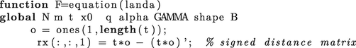
In this appendix a simple Matlab program of nonlinear Example 3 is furnished to ease up the understanding of the proposed method.

Appendix B

Supplementary data

Supplementary data associated with this article can be found, in the online version, athttps://doi.org/10.1016/j.jksus.2020.101288.

Supplementary data

The following are the Supplementary data to this article:

Download

Introduction

Preliminary remarks

Essential results about q-calculus, fractional q-derivatives and q-integrals
Radial basis functions collocation method

Discussion on equivalent problem

Outline of the approximation method

Examination of the method experimentally

Conclusions and future works

Declaration of Competing Interest

Fulltext Views
28

PDF downloads
25

View/Download PDF
Download Citations

BibTeX
RIS

Show Sections

[1] Abdeljawad T., Benli B., Baleanu D., . A generalized q-Mittag-Leffler function by q-Caputo fractional linear equations. Abstr. Appl. Anal.. 2012;2012:1-11.
[Google Scholar]

[2] Abdeljawad T., Baleanu D., . Caputo q-fractional initial value problems and a q-analogue Mittag-Leffler function. Commun. Nonlinear Sci. Numer. Simul.. 2011;16:4682-4688.
[Google Scholar]

[3] Abdeljawad T., Alzabut J., . On Riemann-Liouville fractional q-difference equations and their application to retarded logistic type model. Math. Methods Appl. Sci.. 2018;41:8953-8962.
[Google Scholar]

[4] Agarwal R.P., . Certain fractional q-integrals and q-derivatives. Proc. Camb. Phil. Soc.. 1969;66:365-370.
[Google Scholar]

[5] Akram T., Abbas M., Iqbal A., Baleanu D., Asad J.H., . Novel numerical approach based on modified extended cubic B-spline functions for solving non-linear time-fractional telegraph equation. Symmetry. 2020;12:1154.
[Google Scholar]

[6] Almeida R., Martins N., . Existence results for fractional q-difference equations of order α∈(2,3)) with three-point boundary conditions. Commun. Nonlinear Sci. Numer. Simul.. 2014;19:1675-1685.
[Google Scholar]

[7] Akram T., Abbas M., Riaz M.B., Ismail A.I., Ali N.M., . Development and analysis of new approximation of extended cubic B-spline to the non-linear time fractional Klein-Gordon equation. Fractals. 2020;28:1-20.
[Google Scholar]

[8] Akram T., Abbas M., Riaz M.B., Ismail A.I., Ali N.M., . An efficient numerical technique for solving time fractional Burgers equation. Alex. Eng. J.. 2020;59(4):2201-2220.
[CrossRef] [Google Scholar]

[9] Al-Ghafri Kh.S., . Soliton behaviours for the conformable space-time fractional complex Ginzburg-Landau equation in optical fibers. Symmetry. 2020;12:1-14.
[Google Scholar]

[10] Annaby M.H., Mansour Z.S., . q-Fractional Calculus and Equations. New York: Springer Heidelberg; 2012.

[11] Atangana A., Baleanu D., . New fractional derivatives with non-local and non-singular kernel: theory and applications to heat transfer model. Therm. Sci.. 2016;20:763-769.
[Google Scholar]

[12] Atici F.M., Eloe P.W., . Fractional q-calculus on a time scale. J. Nonlinear Math. Phys.. 2007;14:341-352.
[Google Scholar]

[13] Caputo M., Fabrizio M., . A new definition of fractional derivative without singular kernel. Prog. Fract. Differ. Appl.. 2015;1:73-85.
[Google Scholar]

[14] Feng W., . Exact solutions and conservation laws of time-fractional Levi equation. Symmetry. 2020;12:1-13.
[Google Scholar]

[15] Ghanbari B., Atangana A., . An efficient numerical approach for fractional diffusion partial differential equations. Alex. Eng. J.. 2020;59:2171-2180.
[Google Scholar]

[16] Jackson F.H., . On q-functions and a certain difference operator. Trans. R. Soc. Edinb.. 1908;46:64-72.
[Google Scholar]

[17] Jarad F., Abdeljawad T., Baleanu D., . Stability of q-fractional non-autonomous systems. Nonlinear Anal. Real World Appl.. 2013;14:780-784.
[Google Scholar]

[18] Kac V., Cheung P., . Quantum Calculus. New York: Springer-Verlag; 2002.

[19] Kilbas A.A., Srivastava H.M., Trujillo J.J., . Theory and Applications of Fractional Differential Equations, NorthHolland Mathematics Studies. Vol 207. Amsterdam: Elsevier; 2006.

[20] Al-Mdallal Q.M., Yusuf H., Ali A., . A novel algorithm for time-fractional foam drainage equation. Alex. Eng. J.. 2020;59:1607-1621.
[Google Scholar]

[21] Lyu P., Vong S., . An efficient numerical method for q-fractional differential equations. Appl. Math. Lett. 2019
[CrossRef] [Google Scholar]

[22] Salahshour S., Ahmadian A., Chan C.S., . Successive approximation method for Caputo q-fractional IVPs. Commun. Nonlinear Sci. Numer. Simul.. 2015;24:153-158.
[Google Scholar]

[23] Shi D., Zhang Y., Liu W., . Multiple exact solutions of the generalized time fractional foam drainage equation. Fractals. 2020;28:2050062.
[Google Scholar]

[24] Stynes M., . Fractional-order derivatives defined by continuous kernels are too restrictive. Appl. Math. Lett.. 2018;85:22-26.
[Google Scholar]

[25] Tang Y., Zhang T., . A remark on the q-fractional order differential equations. Appl. Math. Comput.. 2019;350:198-208.
[Google Scholar]

[26] Wang Q., Wang H., . Meshless method and convergence analysis for2-dimensional Fredholm integral equationwith complex factors. J. Comput. Appl. Math.. 2016;304:18-25.
[Google Scholar]

[27] Wang Zh., Zhang L., Li Ch., . Lie symmetry analysis to the weakly coupled kaup-kupershmidt equation with time fractional order. Fractals. 2019;27:1950052.
[Google Scholar]

[28] Wei S., Chen W., Zhang Y., Wei H., Garrard R.M., . A local radial basis function collocation method to solve the variableorder time fractional diffusion equation in a twodimensional irregular domain. Numer. Methods Partial Differ. Equ.. 2018;34:1209-1223.
[Google Scholar]

[29] Wu G.C., Baleanu D., . New applications of the variational iteration method-from differential equations to q-fractional difference equations. Adv. Differ. Equ.. 2013;2013:21-37.
[Google Scholar]

[30] Zhang T., Guo Q., . The solution theory of the nonlinear q-fractional differential equations. Appl. Math. Lett.. 2020;104
[CrossRef] [Google Scholar]

[31] Zhang T., Tang Y., . A difference method for solving the q-fractional differential equations. Appl. Math. Lett.. 2019;98:292-299.
[Google Scholar]

[32] Ain, Q.T., He, J.H., Anjumand, N., Ali, M. The Fractional complex transform: a novel approach to the time-fractional Schrodinger equation. Fractals. doi: 10.1142/S0218348X2150002X.

RBF collocation approach to calculate numerically the solution of the nonlinear system of qFDEs

Abstract

Keywords

q-Fractional derivative

q-Fractional integral

q-Fractional differential equation

Radial basis functions

Collocation method

05A30

39A13

74H20

1 Introduction

2 Preliminary remarks

2.1 Essential results about q-calculus, fractional q-derivatives and q-integrals

2.2 Radial basis functions collocation method

3 Discussion on equivalent problem

4 Outline of the approximation method

5 Examination of the method experimentally

6 Conclusions and future works

Declaration of Competing Interest

References

Appendix A

Appendix B

Supplementary data

Supplementary data

Suggested read for related articles: