

Proposal of an optimization tool for demand response in island electricity systems (IES) using the Simplex method and Generalized reduced gradient (GRG)
⁎Corresponding author. federico.leon@ulpgc.es (Carlos A. Mendieta Pino),
-
Received: ,
Accepted: ,
This article was originally published by Elsevier and was migrated to Scientific Scholar after the change of Publisher.
Abstract
Island electricity generation systems (IES) pose challenges in the integration of renewable energies that are compatible with security of supply. This work proposes a methodology and a proposed decision tool that allows the optimization of the production of different generation systems, both renewable and non-renewable, setting a series of objectives such as the reduction of greenhouse gases (GHG), production costs and at the same time fulfilling the best coverage in dynamic response, security, scalability, and integration. This tool is based on operational research, mathematical optimization methods, specifically the simplex algorithm and the generalized reduced gradient (GRG) and proposes different combinations to achieve an energy production that meets the demand, minimizing fuel consumption and greenhouse gas (GHG) emissions.
Keywords
Simplex method
Generalized reduced gradient algorithm
Optimization model
Energy policy
Renewable energy
Island electricity systems (IESs)

1 Introduction
In previous studies, such as those by (Berna-Escriche et al., 2022), (Papadopoulos, 2020), and (Vargas-Salgado et al., 2022), as well as more recent ones, such as those by (Lozano Medina et al., 2024b), various scenarios have been proposed for studying the transition and challenges faced by an island generation system in the implementation of a more sustainable generation and in parallel a promotion of a greater penetration of renewable energies with guaranteed. Several scenarios have been proposed which allow the transition and challenges faced by an island generation system in the implementation of a more sustainable generation and in parallel a promotion of a greater penetration of renewable energies with guaranteed supply to be studied supply (Kennedy et al., 2017) and (Qiblawey et al., 2022). Conversely, to address the challenges posed by the lack of connectivity in island energy systems (Katsaprakakis, 2016; Paspatis et al., 2023), energy storage systems are proposed (Ferreira et al., 2013), the implementation of energy storage systems by hydroelectric pumping has been proposed for the Canary Islands. One of the most prominent examples of this approach is the PHES project “Chira-Soria.” This system and its integration into the island energy system has been studied by (Lozano Medina et al., 2024a), who concluded that its implementation would maximize the integration of renewable energies. However, they also identified a need for the development of an advanced tool for the optimal selection of systems in the island energy mix. The methodology employed in the analysis of generation in power generation systems has been studied at the continental level (Gkonis et al., 2020; Gómez-Calvet et al., 2019) or at the island level (Paúl Arévalo et al., 2022; Paul Arévalo et al., 2022; Lobato et al., 2017; Sigrist et al., 2017). The Hybrid Optimization of Multiple Energy Resources (HOMER) model (Berna-Escriche et al., 2022; Vargas-Salgado et al., 2022) has been employed in this context. However, it does not consider other scenarios such as existing systems or the use of other types of renewable or lower emission fuels applied in conventional generation systems (Lozano Medina et al., 2024b).Table 1.Table 2.Table 3.Table 4..
| Type Technology | Acronyms |
|---|---|
| Gas Turbine Power | PTG |
| Steam Turbine Power | PTV |
| Combined Cycle Power | PCC |
| 4-Stroke Diesel Engine | PD4T |
| 2-stroke diesel engine | PD2T |
| Power Ranges (MW) | ||||
|---|---|---|---|---|
| Inequality1 | Gas Turbine Power | 2.7 | < PTG < | 125.0 |
| Inequality2 | Steam Turbine Power | 18.0 | < PTV < | 500.0 |
| Inequality3 | Combined Cycle Power | 18.0 | < PCC < | 500.0 |
| Inequality4 | 4-stroke diesel engine power | 1.3 | < PD4T < | 130.0 |
| Inequality5 | 2-stroke diesel engine power | 1.4 | < PD2T < | 45.0 |
| Inequality6 | Power to be covered | PTG + PTV + PCC + PD4T + PD2T = P Total Demandada −P Eólica-P Fotovoltaica | ||
The objective of this study is to develop a tool that relates all the variables of energy production through thermal systems, with the aim of minimizing costs and emissions and covering the energy demand that cannot be covered by energy production through renewables. For the purposes of this study, the 2021 energy data for the island of Gran Canaria and its generation system have been made available (Lozano Medina et al., 2024b). The objective of this tool is to optimize the energy production system using combustion technology (non-renewable) and combine it with energy production using renewables that meet expectations in terms of dynamic response, safety, scalability, and integration with renewable energy systems. The achievement of the objective will be based on operational research, mathematical optimization methods, namely the simplex algorithm (Alekseyev et al., 1990; Hardt et al., 2021; Kasprzyk and Jaskuła, 2004; Msabawy and Mohammad, 2021) and the generalized reduced gradient (GRG) applied in various domains (Haggag, 1981; Msabawy and Mohammad, 2021; Qiu et al., 2022), In 2022, a number of different combinations will be proposed in order to achieve energy production that meets the demand while minimizing fuel consumption and greenhouse gas (GHG) emissions. As a case study and validation of the model, it has been applied to the case of the electricity system of the island of Gran Canaria.
2 Materials and methods
2.1 Methodology
The methodology followed for the achievement of the possible operational improvements sought in the energy generation process has been outlined in Fig. 1.
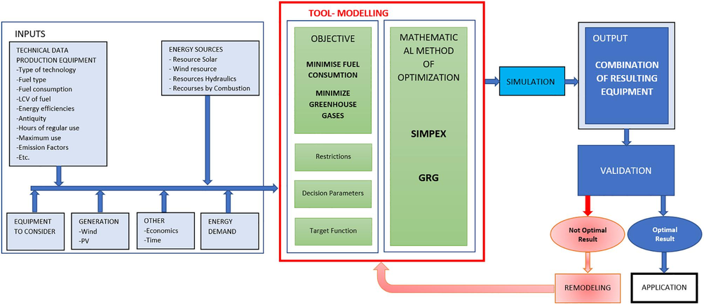
- Methodology.
Operational research will be used to optimize the use of energy production equipment in such a way as to minimize emissions and costs, as well as to assist in the integration of renewable energy. To this end, representative equations of the operation of the equipment are investigated and reproduced, being the representation of this operation a complex and novel work.
2.2 Mathematical methods of optimization. Simplex algorithm and Generalized reduced gradient
Operations Research or management science is a set of tools that are used in mathematical and statistical models to find the best solution, with the objective of helping in decision making. Although this area is very broad and covers various models. For the resolution of the equations, both linear and non-linear, which are raised with the tool, linear programming and non-linear programming will be used respectively, this procedure will focus on the following methods:
-
-
Simplex algorithm. For linear programming with constraints, and more than two variables, where all the expressed terms are going to be linear, the sim-plex algorithm will be used. Operating with linear problems may seem at first very complex, but if the correct steps are followed, the optimal solution will be reached. First identify the decision variables followed by the objective function and finally the constraints. When you have reached this point, you can solve in two ways: numerically or graphically. But to find the solution to this type of problem graphically, you would have to deal with linear models with two variables. For three or more variables, another more specific method of resolution should be applied, such as the method of interior points or the Simplex method. The difference between these two techniques is that if it is applied for interior points, one will operate in the interior of the feasible region while with the Simplex method one will operate with the exterior points of the region, which can take less time to find the optimal solution. The Simplex method is a mathematical practice that, by searching and checking the different solutions, provides the optimal solution of the linear problem.
-
-
Generalized Reduced Gradient, (GRG). For constrained nonlinear programming, a nonlinear optimization code, Generalized Reduced Gradient, will be used. For the optimization of unconstrained nonlinear programming models, there is a category of methods called “General Descent Algorithms”, among which the Gradient Method or Steepest Descent Method (also known as Cauchy Method) stands out, which reduce the computation of a local minimum to a sequence of linear search problems (or one-dimensional search).
2.3 Development of a tool for the study of power scaling in thermal power plants in combination with renewables in isolated island systems
The development of a tool to optimize the power production equipment and describe the different existing combinations to achieve the energy production that satisfies the demand, optimizing a) the cost of fuel, choosing equipment with lower fuel consumption and equipment that operates with the least expensive fuel, b) GHGs, choosing equipment with lower pollution and therefore GHGs (tCO2eq). With this tool it is possible to obtain, for the different energy demands, the best combination of equipment to produce the demanded power with the lowest GHG and the lowest fuel costs. Once the energy consumption data have been analyzed, as well as the technical and operational characteristics of the available combustion energy production equipment, the tool will be developed using mathematical optimization methods, specifically the Simplex method and Generalized Reduced Gradient (GRG) from Operations Research.
2.3.1 Development of a tool for GHG minimization
As already mentioned, the aim is to develop a tool to optimize the choice of power production equipment, with its application to those existing in Gran Canaria, based on their performance, fuel consumption, type of fuel, etc., which reduce GHG. In this case, a linear function to be optimized with linear restrictions is finally obtained, which is why the Simplex optimization method or Simplex algorithm has been used. As already indicated, the tool seeks to optimize fuel consumption and type and therefore minimize GHG emissions. Based on this, the decision variables, the objective functions, and the constraints will be defined.
DECISION VARIABLES: The instantaneous powers of the different production teams were taken as decision variables. This is:
TARGET FUNCTION: In terms of the target function, the aim is to minimize GHG emissions. This objective function defines the hourly emissions of energy production equipment as a function of the installed power or power produced in an hour. To achieve the objective function and determine the decision variables, we work with the emission factor equations of the producing equipment, transforming them until the appropriate objective function is reached. For each type of production technology, the following must be defined:
2.3.2 Application of the Generalized reduced gradient method
As already indicated, the tool seeks to optimize fuel consumption and type and therefore minimize production costs. Based on this, the decision variables, the objective functions, and the constraints will be defined. Taking into account the behaviour of the production equipment, the current energy production of Gran Canaria is supported by 4 steam turbines, 5 diesel equipment, 5 gas turbines, 2 combined cycles with double gas turbine and steam turbine. Among the data studied is the variation of the efficiency (%) versus the instantaneous power (MW) produced, the fuel consumption as a function of its operating regime, type of fuel, etc. To achieve the objective functions, we work with the equations of the power-performance curves of the producing equipment, transforming them until the appropriate objective function is reached.
LOGARITHMIC HIGH CURVE:
LOGARITHMIC LOW CURVE:
HIGH POTENTIAL CURVE:
LOW POTENTIAL CURVE:
DECISION VARIABLES: The instantaneous powers of the different production teams were taken as decision variables. This is:
OBJECTIVE FUNCTION: As for theobjective function, it seeks to minimize production costs, this function defines the economic cost-hour of the energy production equipment based on the installed power or power produced in an hour and its fuel consumption. To achieve the objective functions and determine the decision variables, we work with the equations that relate the performance of the equipment to its production,
Replacing
Logarithmic Target Function:
3 Results
3.1 Simplex method
3.1.1 Application of the tool to minimise hourly emissions of energy production equipment
The developed tool is applied. It is analyzed 24 h a day on August 17, 2021, the day when the highest annual energy demand occurred at 2:53p.m., with 529.0 MW of instantaneous power. In this case, as already indicated, the tool seeks to minimize GHGs. As a result of this application, in the 24 h we have a combination of power-producing equipment that makes emissions as low as possible, meeting the energy demand. The following graph shows, among others, the “GHG” curve that indicates the actual emissions produced during the 24 h and the “GHG Minimized” curve, emissions produced by the best combination of equipment based on the restrictions and methodology established by the tool.
The algorithm established a new combination (it exclusively chose combined cycle technology for energy production), which decreases emissions in 24 h by 388.0 tCO2eq, (8.83 %). In Fig. 2, in addition to representing the two curves: “GHG”, which are the actual emissions produced on August 17, 2021, and “GHG Minimized”, which represent the emissions that would have occurred on August 17, 2021 if the combination of equipment proposed by the algorithm to minimize GHGs had been used, The “GHG for Minimized cost” curve is also represented, which indicates the GHG emissions that would have occurred on August 17, 2021 if the combination of equipment proposed by the algorithm had been used to minimize costs. As will be seen in the corresponding section, cost minimization involves another combination of different equipment and therefore a different GHG production. This new combination of technologies results in a 24-hour decrease in GHGs by 338.3 tCO2eq (7.61 %).Fig. 3..
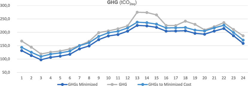
- GHG emissions.
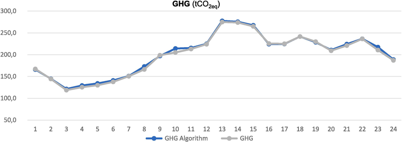
- Comparison of real GHG vs. estimated by the GHG Algorithm.
3.1.2 Model validation to minimise emissions
When we have obtained the optimal solution to the system, we must validate the model, that is, check if the result obtained makes sense and the decisions can be executed ((Mathur et al., 1996)). Therefore, we will determine whether to accept the model and then apply it later or reject it in such a way that we will have to rework the modelling process. To determine the validity of the system, we will analyze the agreement between the observed data of the real model and those provided by the model (Ríos-Insua et al., 2006) by choosing the combination of equipment that was used in the real model and running the algorithm with this combination, and then comparing results. To validate the model determined to search for the minimum emissions, different simulations have been made with the simplex method of different combinations of operation of the production equipment, for which real emissions data are available and the differences between the algorithm and reality have been verified. The percentage of deviation has been estimated, all of which are less than 1.00 %. An example is the validation study that was carried out where the emissions produced on August 17, 2021 were studied.
It has been verified that the real GHG on that day was 4,781.0 tCO2eq and those estimated by the algorithm 4,828.3 tCO2eq, which is a 0.979 % deviation. Therefore, the tool for GHG estimation is considered validated.
3.2 Generalized reduced gradient method
3.2.1 Application of the tool to minimize energy production costs
The developed tool is applied. In the case of the logarithmic objective function, coherent results are not obtained and it is not applicable to the system followed, so we will work with the potential objective function that did give good results.
It is analyzed 24 h a day on August 17, 2021, the day when the highest annual energy demand occurred at 2:53p.m., with 529.0 MW of instantaneous power. In this case, as already indicated, the tool seeks to minimise the economic cost of energy production equipment depending on the installed power and/or production demanded. As a result of this 24-hour application, a combination of power-producing equipment is produced that makes the economic cost as low as possible while meeting the energy demand. The following graph shows, among others, two curves that indicate the real costs during the 24 h and the costs established by the tool, algorithm, with its new combination of producing equipment.
The algorithm established a new combination (it chose the combined cycle and two-stroke diesel engine technologies for energy production), which decreases the cost in 24 h by €56,015.3, (10.48 %). Fig. 4, in addition to representing the “Cost” curves, which are the actual costs incurred on August 17, 2021, and the “Cost Minimized” curves, which represent the costs that would have occurred on August 17, 2021 if the combination of equipment proposed by the algorithm had been used to minimize them, the “Cost to Minimized GHGs” curve is also represented“, which indicates the economic cost that would have occurred on 17 August 2021 if the combination of equipment proposed by the algorithm had been used to minimise GHGs. As seen in previous sections, GHG minimization involves another combination of different equipment and therefore another production of different costs. This new combination of technologies means a reduction in costs in 24 h by €49,255.3, (9.10 %).Fig. 5..
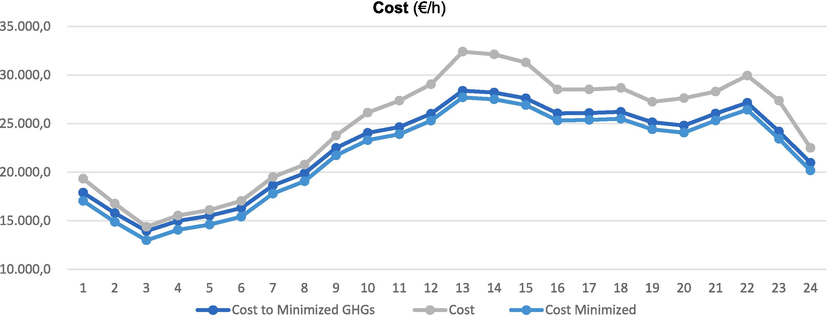
- Economic costs.
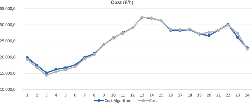
- Comparison of actual fuel consumed costs versus those estimated by the algorithm.
3.2.2 Model validation to minimize economic cost
To validate the model determined to find the minimum fuel consumption, the most economical and most profitable, simulations have been made with the method of the generalized reduced gradient of operating data of the production equipment and the differences between the algorithm and reality have been verified, estimating the percentage of deviation, all of which are less than 1.00 %. An example is the validation study that was carried out where the costs produced on August 17, 2021 were studied.
It has been verified that the actual costs on that day were €590,416.9 and those estimated by the algorithm were €592,532.9, which represents a 0.357 % deviation. Therefore, the tool for estimating the cost of fuel consumption is considered validated.
3.2.3 Combined solution. Application to minimise energy production costs and GHGs
Fig. 4, as already indicated, also shows a third curve: “Cost to Minimized GHGs”, with which the costs produced by the combination of equipment that produce lower GHGs have been represented. As you can see, it improves the costs of the real case, and equalizes the costs of the best existing combination to minimize them. On the other hand, in Fig. 2, a third curve is also shown: “GHG for Minimized cost”, with this curve the GHGs produced by the combination of equipment that produces lower costs has been represented. As can be seen, it improves the GHGs of the real case, and equalizes the minimized GHGs.
4 Summary of applied methods
With all this, it is obtained, in summary, that the maximum daily cost savings in fuels in power production plants can be estimated for the day studied of approximately €85,000, if we choose exclusively to minimize the cost. And it has been obtained that the maximum daily decrease of GHGs in power production plants can be estimated to be approximately 388 tCO2eq for the day studied, if we choose exclusively to minimize GHGs as shown in Table 5.
| Algoritmo | Real data | Real Combination of Technologies simulated with the algorithm |
Combining technologies for get the Minimized Cost |
Combining technologies for obtain the Minimized GHG |
|||
|---|---|---|---|---|---|---|---|
| amount | amount | % Difference from Actual |
amount | % Difference from Actual |
amount | % Difference from Actual |
|
| GHG (tCO2eq) | 4,781.0 | 4,828.3 | 0.979 % | 4,442.7 | −7.616 % | 4,393.0 | −8.833 % |
| Cost (€) | 590,416.9 | 592,532.9 | 0.357 % | 534,401.6 | −10.482 % | 541,161.7 | −9.102 % |
5 Discussion and conclusions
The algorithm represents a valid tool for the management of production teams, offering the optimal combination of these teams for the optimal optimisation of the variable in the studio. The algorithm and methodology have been employed to resolve the dual problem posed, with operations research serving as the precursor to programming. This mathematical tool has enabled us to develop our problem with continuous variables and linear constraints. Indeed, alternative methods have been employed to address these issues, which can be analysed or visualised. The graphical method is arguably one of the most expedient and transparent approaches to problem-solving. However, it is limited in its applicability to scenarios involving only two variables, a constraint that is seldom encountered in real-world contexts. This is where the relevance of both methods becomes apparent. The algorithm has been demonstrated to be effective even when the number of variables is high, as long as there is at least one variable. Consequently, it can be posited that the Simplex and GRG methods are capable of providing an optimal solution to the decision-making process, as they consistently identify the optimal value that maximises the target function. In the case under analysis, two individual solutions were obtained in accordance with the objective sought, and a third of compromise was also identified.
-
The optimal solution for the optimisation of production equipment in order to reduce costs was identified, resulting in a cost reduction of 9.102 %.
-
The optimal configuration of production equipment for the reduction of GHG emissions, resulting in a decrease in GHG of 8.833 %. The aforementioned methods have been demonstrated to markedly enhance the outcomes of the equipment combination selected by the production company.
-
Conversely, it has also served to seek a third compromise solution, which encompasses the two joint optimisations of cost and GHG, resulting in a superior compromise solution to that applied by the producing company. This solution comprises an alternative combination of equipment that offers the lowest economic cost, as illustrated in Fig. 4. This combination is comparable to the one that minimises GHGs the most, although it is slightly above this minimum. The GHG curve for the Minimised COST, represented in Fig. 2, shows that this combination of equipment produces GHGs that are well below those produced by the solution adopted by the producing company.
Funding
This research was cofunded by the INTERREG V-A Cooperation, Spain–Portugal MAC (Madeira-Azores-Canaries) 2014–2020 program, MITIMAC project (MAC2/1.1a/263).
CRediT authorship contribution statement
Juan Carlos Lozano Medina: Writing – review & editing, Writing – original draft, Visualization, Validation, Supervision, Software, Resources, Methodology, Investigation, Formal analysis, Data curation, Conceptualization. Vicente Henríquez Concepción: Visualization, Validation, Supervision. Carlos A. Mendieta Pino: Writing – review & editing, Writing – original draft, Visualization, Validation, Supervision, Investigation, Funding acquisition, Conceptualization. Federico León Zerpa: Writing – review & editing, Validation, Supervision, Resources.
Declaration of Competing Interest
The authors declare the following financial interests/personal relationships which may be considered as potential competing interests: [Carlos Alberto Mendieta Pino reports was provided by University of Las Palmas de Gran Canaria. Carlos Alberto Mendieta Pino reports a relationship with University of Las Palmas de Gran Canaria that includes: employment. If there are other authors, they declare that they have no known competing financial interests or personal relationships that could have appeared to influence the work reported in this paper].
References
- Application of the resolving multipliers of the modified simplex method in problems of integer linear programming. USSR Comput. Math. Math. Phys.. 1990;30:114-115.
- [CrossRef] [Google Scholar]
- Can a fully renewable system with storage cost-effectively cover the total demand of a big scale standalone grid? analysis of three scenarios applied to the Grand Canary Island, Spain by 2040. J. Energy Storage. 2022;52:104774
- [CrossRef] [Google Scholar]
- Characterisation of electrical energy storage technologies. Energy. 2013;53:288-298.
- [CrossRef] [Google Scholar]
- Multi-perspective design of energy efficiency policies under the framework of national energy and climate action plans. Energy Policy. 2020;140:111401
- [CrossRef] [Google Scholar]
- Current state and optimal development of the renewable electricity generation mix in Spain. Renew. Energy. 2019;135:1108-1120.
- [CrossRef] [Google Scholar]
- A variant of the generalized reduced gradient algorithm for non-linear programming and its applications. Eur. J. Oper. Res.. 1981;7:161-168.
- [CrossRef] [Google Scholar]
- Investigations on the application of the downhill-simplex-algorithm to the inverse determination of material model parameters for FE-machining simulations. Simul. Model. Pract. Theory. 2021;107:102214
- [CrossRef] [Google Scholar]
- Application of the hybrid genetic-simplex algorithm for deconvolution of electrochemical responses in SDLSV method. J. Electroanal. Chem.. 2004;567:39-66.
- [CrossRef] [Google Scholar]
- Hybrid power plants in non-interconnected insular systems. Appl. Energy. 2016;164:268-283.
- [CrossRef] [Google Scholar]
- Optimal hybrid power system using renewables and hydrogen for an isolated island in the UK. Energy Procedia. 2017;105:1388-1393.
- [CrossRef] [Google Scholar]
- Value of electric interconnection links in remote island power systems: the Spanish canary and balearic archipelago cases. Int. J. Electr. Power Energy Syst.. 2017;91:192-200.
- [CrossRef] [Google Scholar]
- A case study of a reverse osmosis based pumped energy storage plant in canary islands. Water (basel). 2024;16
- [CrossRef] [Google Scholar]
- Alternatives for the optimization and reduction in the carbon footprint in island electricity systems (IESs) Sustainability. 2024;16
- [CrossRef] [Google Scholar]
- Management science: the art of decision making, Investigación de operaciones: el arte de la toma de decisiones. Englewood Cliffs, N.J.: Prentice Hall; 1996.
- Continuous sizing optimization of cold-formed steel portal frames with semi-rigid joints using generalized reduced gradient algorithm. Mater. Today: Proc.. 2021;42:2290-2300.
- [CrossRef] [Google Scholar]
- Renewable energies and storage in small insular systems: potential, perspectives and a case study. Renew. Energy. 2020;149:103-114.
- [CrossRef] [Google Scholar]
- Assessment of the required running capacity in weakly interconnected insular power systems. Electr. Pow. Syst. Res.. 2023;221:109436
- [CrossRef] [Google Scholar]
- Qiblawey, Y., Alassi, A., Zain ul Abideen, M., Bañales, S., 2022. Techno-economic assessment of increasing the renewable energy supply in the Canary Islands: The case of Tenerife and Gran Canaria. Energy Policy 162, 112791. doi: 10.1016/j.enpol.2022.112791.
- Generalized Extreme Gradient Boosting model for predicting daily global solar radiation for locations without historical data. Energy Convers. Manag.. 2022;258:115488
- [CrossRef] [Google Scholar]
- A multi-attribute decision support system for selecting intervention strategies for radionuclide contaminated freshwater ecosystems. Ecol. Model.. 2006;196:195-208.
- [CrossRef] [Google Scholar]
- Economic assessment of smart grid initiatives for island power systems. Appl. Energy. 2017;189:403-415.
- [CrossRef] [Google Scholar]
- Optimization of the electricity generation mix using economic criteria with zero-emissions for stand-alone systems: case applied to Grand Canary Island in Spain. Prog. Nucl. Energy. 2022;151:104329
- [CrossRef] [Google Scholar]
Appendix A
Supplementary material
Supplementary data to this article can be found online at https://doi.org/10.1016/j.jksus.2024.103345.
Appendix A
Supplementary material
The following are the Supplementary data to this article:


