

Translate this page into:
Porosity prediction based on LS-SVR: A case study in Shuangcheng depression of the Northern Songliao Basin
*Corresponding author E-mail address: yrz@cumtb.edu.cn (R. Yang)
-
Received: ,
Accepted: ,
Abstract
Porosity is a key indicator for evaluating reservoir quality. Porosity analysis identifies the type, structure, and distribution of reservoir pores, essential for evaluating oil and gas accumulation and reserves. Accurately predicting porosity is crucial for petroleum exploration and engineering in the Shuangcheng Depression, Northern Songliao Basin. Traditional methods, such as core sampling, are often limited by high costs, time constraints, and the need for discrete samples that may not fully represent the reservoir, thereby hindering accurate porosity prediction. Therefore, this study assesses the accuracy of porosity prediction using the Least Squares Support Vector Regression (LS-SVR) model, selected for its effectiveness in handling small datasets and capturing nonlinear relationships. LS-SVR also mitigates computational challenges associated with traditional Support Vector Regression (SVR). The model utilizes geological and geophysical data from the Shuangcheng Depression in the southeastern fault zone of the Northern Songliao Basin to predict reservoir porosity. Nine well-logging data are used as input features, with porosity values obtained from core samples serving as the target label. This study develops an optimal porosity prediction model by training it with a sigmoid function, optimizing the penalty factor C and kernel parameter γ via grid search, and selecting the best parameters through 5-fold cross-validation. To ensure the model's performance, statistical metrics are used to evaluate the model. Evaluation results show that the model achieves an R2 of 0.90 on the test set, explaining 90% of the variance in the target variable. Compared to traditional methods, the LS-SVR model demonstrates a significant improvement in porosity prediction. The remaining metrics include MAE (0.55), MSE (0.40), and RMSE (0.63). The results indicate that the LS-SVR method significantly improves the prediction of reservoir porosity in the Shuangcheng Depression of the Northern Songliao Basin. It is crucial for reservoir evaluation and petroleum engineering decision-making, providing valuable references for further research and practical applications.
Keywords
Feature selection
LS-SVR
Machine learning
Model evaluation
Parameter optimization
Porosity

1. Introduction
In petroleum reservoir characterization, predicting reservoir properties is critical to evaluation research, and porosity is a vital parameter for quantifying the void space in rocks (Oluwadamilola Olutoki et al., 2024). Accurately estimating porosity is essential for reservoir modeling, well placement selection, and production optimization (Alatefi et al., 2023). Traditional laboratory analysis of core samples is regarded as the most accurate method for porosity estimation. However, it is not always feasible. Subsurface geological conditions are highly variable and complex. Each well faces unique challenges during the coring process, leading to potential difficulties in sample analysis (Ahmadi and Chen, 2019). Additionally, core sampling provides discrete samples from the drilling process, which may not fully reflect the characteristics of the entire reservoir. Establishing regression relationships between well-logging curves and reservoir parameters has become a widely used method in reservoir evaluation. Well-logging data can address the issue of discontinuous core information. However, this method relies on empirical relationships and may struggle to adapt to the complexity and heterogeneity of reservoirs. Furthermore, logging data gaps may exist, introducing uncertainty and challenges to geological interpretation (Xiao et al., 2020), reservoir evaluation, and oil and gas exploration decisions. a novel approach is urgently needed to overcome these challenges (Newman et al., 1977; Byrnes et al., 1994; Wu et al., 2004).
Advancements in machine learning and computing now enable nonlinear techniques to analyze the distribution characteristics of simulated underground reservoir porosity. These techniques can quickly solve large-scale mathematical computation problems and meet the scientific requirements for reservoir feature identification in oil and gas exploration (Xie et al., 2017; Dong et al., 2016; Othman and Gloaguen; 2017, Zhong et al., 2020). Artificial Neural Networks (ANN) are powerful tools for predicting reservoir properties from well-logging data, effectively capturing complex relationships within the data (Anifowose et al., 2017). Urang et al. proposed a method using neural networks to predict reservoir physical parameters, including porosity and permeability, which was applied in the Niger Delta, Nigeria (Urang et al., 2020). However, ANN may suffer from overfitting when dealing with small sample sizes, resulting in poor interpretability of the generated results. Support Vector Machines (SVM) overcome the challenges of complex model structures and parameter selection often encountered in traditional neural networks (Behnoud far et al., 2017; Konaté et al., 2015; Rafik and Kamel, 2017). SVM, proposed by Boser et al., has been successfully applied to classification problems (Boser et al., 1992; Cortes et al., 1995). Nevertheless, predicting porosity values is a regression problem that requires handling large-scale datasets and demands a higher level of interpretability for the results. Therefore, a variant of SVM, known as Support Vector Regression (SVR), is more suitable in this context.
SVR, as a statistical-based method of SVM regression, exhibits better nonlinear modeling capability, generalization ability, and interpretability, making it suitable for predicting reservoir properties (Wang et al., 2023a). Numerous researchers have achieved significant results in predicting reservoir porosity and physical parameters using Support Vector Machine regression. For instance, Wang et al. applied the SVR model to evaluate reserve abundance, effectively addressing a key challenge in petroleum exploration and development (Wang et al., 2023b). Kor et al. evaluated the applicability of the SVR model for predicting reservoir physical parameters by controlling the sample size. The results demonstrated that SVR can generate better prediction results when the training samples are appropriately increased (Kor and Altun, 2020). Bagheri et al. utilized a radial basis function-based SVR method to estimate permeability in the South Pars gas field, Iran. The evaluation results revealed the accuracy and effectiveness of this approach (Bagheri and Rezaei, 2019). However, solving SVR involves addressing a convex quadratic optimization problem, which can be challenging (Zhu and Gao, 2018, Bermúdez et al., 2019).
To simplify the solution process and enhance the model's predictive capability, this paper proposes the Least Squares Support Vector Regression (LS-SVR) method. The inequality constraints are converted into equality constraints, and the loss function is modified from error to a sum of squared errors. Specifically, the proposed LS-SVR algorithm performs modeling and prediction by mapping the input space to a high-dimensional feature space to derive the optimal linear function. LS-SVR has been widely applied in fields such as geophysics and geological engineering. Its ability to address computational challenges in traditional SVR makes it particularly suitable for these domains. For instance, in 2024, Wei Cong integrated LS-SVR with other machine learning models to enhance the accuracy of predicting CH4 and C2Hn generated during the gasification process, contributing to the reduction of pollutant emissions, waste, and greenhouse gases (Cong, 2024). Additionally, Chen et al. proposed an Attention-Weighted LS-SVR Regression method for predicting carbon prices, using attention mechanisms to create a weight matrix for variables, thereby enhancing the model's performance (Chen and Zhao, 2024). In this study, the LS-SVR model demonstrates good predictive capability for porosity prediction using geophysical well logging data. It performs well on evaluation metrics such as Mean Absolute Error (MAE), Mean Squared Error (MSE), Root Mean Squared Error (RMSE), and Coefficient of Determination (R2), as shown in Table 1. These results highlight the robustness and versatility of LS-SVR in addressing complex prediction tasks across diverse domains.
| LS-SVR model | Parameters | Test | |||
| C search range | [0.01, 0.1, 1, 10, 100] | MAE | MSE | RMSE | R2 |
| γ search range | [0.001, 0.01, 0.1, 1, 10, 100] | ||||
| Test set sample number | 212 | 0.55 | 0.40 | 0.63 | 0.90 |
MSE: Mean squared error, MAE: Mean absolute error, RMSE: Root mean squared error, Coefficient of determination (R2).
2. Geological setting
The study area is in the southeastern fault zone of the Beicheng Depression, which lies within the northern Songliao Basin. Geogra-phically, it is situated within the jurisdiction of Shuangcheng City, Harbin City, Heilongjiang Province. Fig. 1(a) shows the geographical location of the Shuangcheng Depression, highlighted with a red border, providing context for the study area's position within the Songliao Basin. The southern part of the Shuangcheng Depression is connected to the Yushu fault zone in Jilin, while the western part is adjacent to the Duqingshan uplift and the Yingshan depression. It is influenced by the Taipingzhuang and Chaoyang faults, with an exploration area of 1031 km2 within the fault-controlled area. Fig. 1(b) presents a schematic diagram of the structural features of the Shuangcheng Depression. The black border outlines the study area, showing its position relative to the surrounding tectonic boundaries. The diagram emphasizes the exploration area of 1031 km2. In terms of structural trends, the southeastern region of the study area is a deeper, subsiding depression, while the central part is characterized by an uplifted region, forming a north-northeast-dipping axial syncline. The northwest slope represents a transition to a shallower area, where subsidence decreases, and the terrain gradually becomes less depressed. This pattern reflects regional variations in subsidence and elevation, with the southeastern depression being the lowest point and the northwest slope gradually rising in elevation. The faults in the study area show inherited development, suggesting the reactivation of older fault zones from earlier geological periods. These reactivated faults often influence reservoir properties by creating heterogeneity in the subsurface, leading to variations in porosity and permeability. The movement along these faults can result in localized compaction, fracturing, or the creation of barriers that affect fluid flow and storage capacity in the reservoir. The main structures are along the active fault zones within the area, while the central uplift region represents a north-northeast-dipping axial syncline. Fig. 1(c) provides a detailed tectonic map of the study area, highlighting major fault lines, the structural framework, and the distribution of core wells (marked as black circles). The figure illustrates how faults and structural highs influence well placement and reservoir characteristics. The core wells are predominantly located in structurally significant areas (Chen, 2021).

- Regional geological background of the study area. (a) Geographical location of the Shuangcheng Depression in the southeastern fault area of the Beicheng Depression within the northern part of the Songliao Basin (the specific location of the Shuangcheng Depression is indicated by the red border). (b) A schematic diagram of the Shuangcheng Depression structure and the study area, with the specific location of the study area outlined by a black border. (c) Tectonic map of the study area and the distribution of core wells.
In this study, the geological and geophysical data from the Shuangcheng Depression within the southeastern fault area of the Beichengnan Depression in the Songliao Basin was used, provided by the China National Petroleum Corporation. This dataset includes nine well-logging features distributed in the Central Uplift and Southeast Trough area (drilling locations can be seen in Fig. 1c), encompassing logging curve data and lithology interpretation data. Statistical analysis of core test data indicates that the Upper Sandstone Formation mainly comprises sandstone and siltstone, with porosity ranging from 10.1% to 20.9%. Most porosity values fall between 11% and 18%, with an average porosity of 14.29% (Fig. 2).
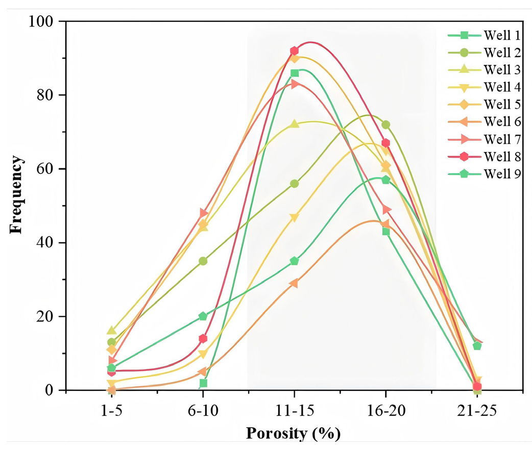
- Porosity distribution characteristics of core well logging (Each curve represents the porosity distribution of an individual well, and the gray area represents the porosity distribution characteristics of the reservoir in the Upper Sandstone Formation; The gray area in the figure represents the average trend of porosity distribution, reflecting the range of porosity variation within the sandstone layer of the reservoir).
3. Working principle of LS-SVR
LS-SVR is a modified version of the standard SVR Model. In LS-SVR, squared error terms replace slack variables in the objective function, transforming the optimization problem from quadratic programming to a system of linear equations. This makes LS-SVR computationally efficient and suitable for tasks that require high-dimensional mapping and regression.
Given a training set , where xi is the input feature vector, yi is the target output, and n is the number of training samples. LS-SVR constructs a regression model in the form (Vapnik et al., 1997):
In (1), w is the parameter vector, b is the bias term, and is a nonlinear mapping function that projects the input x into a high-dimensional feature space. The LS-SVR approach minimizes a squared error-based objective function with equality constraints, as opposed to inequality constraints, which distinguishes it from standard SVR (Li, 2022). In LS-SVR, grid search is used to determine the optimal penalty factor C and kernel parameter γ. The use of squared error simplifies the optimization problem, transforming it into a linear system of equations, which enhances the efficiency of solving the model.
The optimization problem is formulated as follows:
Subject to:
γ is the regularization parameter that controls the trade-off between model complexity and fitting error, ei is the error term associated with the i-th sample.
The optimization problem is solved by applying the method of Lagrange multipliers. The Lagrangian function is constructed as:
where ai are the Lagrange multipliers associated with each equality constraint.
Using the Karush-Kuhn-Tucker (KKT) conditions, we obtain the following system of equations:
Substituting these conditions back into the Lagrange equation gives:
where represents the kernel matrix, is the kernel function, which could be a Gaussian (RBF) kernel or another suitable kernel, allowing nonlinear relationships to be captured.
In the dual form, the regression function is expressed as:
Here, the kernel function can be defined as , where σ is a parameter controlling the width of the kernel.
4. Data and method
The workflow for predicting porosity using the LS-SVR method can be divided into four steps (Fig. 3):
-
1.
Process and optimize the data, then randomly split it into a training set (70%), a validation set (15%), and an independent test set (15%).
-
2.
Select an appropriate kernel function and define hyperparameter search ranges: C = [0.01, 0.1, 1, 10, 100] and γ = [0.001, 0.01, 0.1, 1, 10, 100].
-
3.
A five-fold cross-validation is conducted on the training set to optimize LS-SVR model parameters. In each iteration, one subset is for validation, and the other four are for training. This repeats five times, averaging performance to determine the best hyperparameter combination. The final model, after cross-validation tuning, is evaluated on an independent test set to assess its generalization performance.
-
4.
Evaluate the model using metrics like MAE, MSE, RMSE and R2. The test set assesses its ability to generalize and validate predictive performance.

- (a) The characteristic data (well logs) from 9 wells (Well 1-Well 9 representing different wells) were preprocessed and randomly split into three subsets: a training set (70%), a validation set (15%), and an independent test set (15%). Different well logging curves reflect distinct reservoir lithology characteristics, enabling the model to learn diverse geological features and evaluate its performance across varying subsurface conditions. (b) The preprocessed data (pink circles) were input into the LS-SVR model. Grid search combined with five-fold cross-validation was used to identify the optimal hyperparameters. This process ensures the model captures nonlinear relationships between input data and labels, avoiding biases observed in simpler models. (c) After hyperparameter tuning via cross-validation, the final LS-SVR model was retrained on the combined training and validation sets and rigorously evaluated on the independent test set to assess generalization performance. (d) Model performance was quantified using metrics including MSE, MAE, RMSE, and R2. All metrics were calculated exclusively on the test set to ensure unbiased evaluation. LS-SVR: Least squares support vector regression.
4.1 Data analysis and feature selection
4.1.1 Data analysis
Before establishing the model, compensated neutron porosity (ΦN), core porosity (Φ), and density porosity (ΦD) were collected for comparison (ΦD) (Table 2). The purpose of this analysis was to evaluate and validate the accuracy and reliability of the current porosity calculation methods. Porosity is a crucial parameter in underground reservoirs and has a significant impact on geological research and engineering decision-making. If the calculation methods used have accuracy or reliability issues, the predicted porosity may deviate significantly from the actual conditions, leading to misleading results and inaccurate geological interpretations. This would have negative implications for subsequent geological research and engineering design, potentially resulting in suboptimal engineering outcomes.
| Well | ΦN Min (%) | ΦN Max (%) | ΦD Min (%) | ΦD Max (%) | Φ Min (%) | Φ Max (%) |
| Well 1 | 14.5 | 27.2 | 16.26 | 32.53 | 9.10 | 18.90 |
| Well 2 | 13.95 | 52.02 | 5.00 | 41.51 | 3.00 | 19.60 |
| Well 3 | 12.16 | 22.85 | 8.53 | 26.51 | 1.90 | 22.10 |
| Well 4 | 13.07 | 19.89 | 8.18 | 16.67 | 4.90 | 22.20 |
| Well 5 | 11.19 | 30.00 | 3.01 | 50.00 | 2.30 | 21.50 |
| Well 6 | 14.99 | 24.53 | 10.90 | 35.60 | 8.30 | 23.19 |
| Well 7 | 10.50 | 20.32 | 1.56 | 24.81 | 2.90 | 22.90 |
| Well 8 | 9.57 | 23.78 | 7.23 | 35.54 | 1.00 | 21.70 |
| Well 9 | 11.10 | 24.30 | 1.81 | 39.76 | 2.40 | 23.90 |
Density is linked to rock porosity and mineral composition, and density logging is a commonly method for porosity calculation in log analysis. This method involves measuring the density of the formation to calculate porosity.
First, the reservoir shale content (Vsh) is calculated based on the natural gamma ray log (GR) curve, using empirical formulas:
In the formula, a represents the calibration coefficient. Based on the information provided from the study area, the calibration coefficient is chosen as 0.967. GR represents the measured natural gamma ray value in API units. GRmin and GRmax represent the minimum and maximum GR values in API units. Vsh represents the shale content, expressed as a decimal fraction.
Next, the density porosity is calculated using the empirical formula known as the Wylie formula (ΦD):
In the formula, represents density porosity, expressed as a decimal fraction. is the rock matrix density value, which is 2.66 g/cm3. is the formation fluid density value, which is 1 g/cm3. DEN represents the density logging value for the target formation, measured in g/cm3. is the density of shale, measured in g/cm3. represents the shale content in the reservoir, expressed as a decimal fraction.
Next, ΦD, ΦN, and Φ are compared and analyzed. From Fig. 4, it can be observed that the R2 value between compensated ΦN and Φ is 0.41, with an MSE of 6.84. The R2 value between density porosity and core porosity is 0.33, with an MSE of 2.54. These results may be attributed to the limitations of the calculation methods and the influence of empirical relationships.

- Error analysis of compensated neutron porosity, density porosity, and core porosity. (a) Analysis of errors between neutron porosity and core porosity. (b) Analysis of error between compensated density porosity and core porosity.
4.1.2 Feature selection
In this study, 9 kinds of logging curves and core porosity were collected, including Core porosity (Φ), Caliper Log (CAL), Compensated neutron log (CNL), Density (DEN), Gamma (GR), Laterolog Deep (LLD), Laterolog Shallow (LLS), Resistivity (RT), Spontaneous potential (SP), Acoustic (AC) for statistical analysis. Table 3 presents the dataset's statistical summary, including sample count, average, minimum, and maximum values.
| Features | CAL (cm) | CNL (%) | DEN (g/cm3) | GR (API) | LLD (Ω·M) | LLS (Ω·M) | RT (Ω·M) | SP (mv) | AC (us/m) | Φ (%) |
| Count | 1410 | 1410 | 1410 | 1410 | 1410 | 1410 | 1296 | 1410 | 1410 | 1410 |
| Min | 8.09 | 9.57 | 1.83 | 49.71 | 5.45 | 6.40 | 4.85 | 3.71 | 186.22 | 1.00 |
| Max | 31.08 | 52.03 | 2.63 | 377.00 | 71.95 | 86.12 | 106.99 | 313.92 | 321.81 | 23.90 |
| Average | 10.52 | 17.59 | 2.32 | 117.19 | 21.99 | 23.97 | 22.86 | 129.27 | 240.81 | 14.29 |
To mitigate the risk of high dimensionality and overfitting of the input data, a refined selection of well-logging sequences was made. Fig. 5 shows the correlation matrix of nine well-logging parameters with Φ. CAL shows strong collinearity with SP and RT (correlation coefficients: 0.69, 0.48). RT is also highly correlated with LLS and LLD (0.69, 0.76). Thus, GR, SP, CNL, AC, DEN, and RT are selected to predict porosity.
4.2 Model design
Empirical and experimental methods are utilized for parameter selection during this process. First, a rough parameter range search is conducted to determine the approximate range of parameters. Subsequently, a more detailed optimization is performed within this range. Prior knowledge and domain expertise help select initial parameters, enhance training, and improve model performance.
When selecting parameters, the focus is on the kernel parameter and penalty factor (C) Kernel options include linear, polynomial (poly), Gaussian (rbf), and sigmoid. The penalty factor (C) controls model complexity and penalizes training errors. A grid search is performed within the predefined parameter range to exhaustively explore and identify the optimal parameters (kernel parameters and penalty factor, C) (Fayed and Atiya, 2019). Subsequently, a five-fold cross-validation search for optimal parameter values within the specified range (Fig. 6; (Wang et al., 2023)). Through this parameter tuning process, a relatively optimal model configuration can be obtained (Jung, 2017).

- Correlation matrix plot of nine well logging parameters and porosity.

- Implementation process of 5-fold cross-validation.
5. Results and discussion
5.1 Results
5.1.1 Data set partitioning results
Based on the requirements of the problem and the relevance of the features, the most representative and predictive features were selected. To improve the model's training and generalization, highly correlated features were excluded through correlation analysis, thereby reducing feature dimensionality and preventing redundancy or collinearity among inputs. This ultimately enhances model performance. By calculating Pearson correlation coefficients between different well-logging curves, the linear relationship strength can be assessed. If certain curves exhibit weak or close-to-zero correlation, it indicates that they are independent in providing information and can serve as independent input features. As shown in Fig. 5, the correlation between the six well-logging data is weak. Consequently, the well logging data of Gamma (GR), Density (DEN), Acoustic (AC), Laterolog Deep (LLD), Compensated neutron log (CNL), and Spontaneous potential (SP) can be used as input features for porosity prediction. The entire dataset was divided into a training set (70%), a validation set (15%), and a test set (15%) based on the number of sample labels (Table 4). Prior to dataset partitioning, it is important to eliminate outliers from the collected data to maintain quality and accuracy and prevent the influence of noise on model training. The results indicate that the data fall within the normal range, with no outliers or missing values (Fig. 7).
| Sample | Train numbers | Test numbers | Validation numbers | Amount |
| Well 1 | 91 | 20 | 20 | 131 |
| Well 2 | 124 | 26 | 26 | 176 |
| Well 3 | 136 | 29 | 29 | 194 |
| Well 4 | 89 | 19 | 19 | 127 |
| Well 5 | 146 | 31 | 31 | 208 |
| Well 6 | 44 | 10 | 10 | 64 |
| Well 7 | 141 | 30 | 30 | 201 |
| Well 8 | 125 | 27 | 27 | 179 |
| Well 9 | 90 | 20 | 20 | 130 |
| Amount | 986 | 212 | 212 | 1410 |
| Percent | 70% | 15% | 15% | 100% |
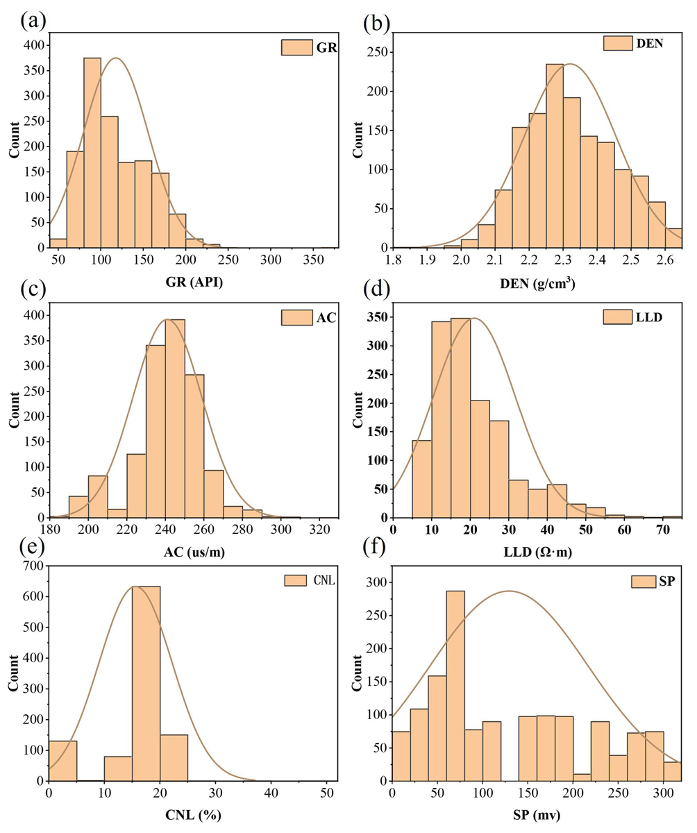
- Distribution of well logging curve values. GR: Gamma, DEN: Density, AC: Acoustic, LLD: Laterolog deep, CNL: Compensated neutron log, SP: Spontaneous potential.
5.1.2 Results of parameter selection and training
Firstly, experiments in LS-SVR were conducted using different kernel functions, including the linear kernel, polynomial kernel, Gaussian kernel (rbf), and sigmoid kernel. These experiments compared the performance of the linear kernel, polynomial kernel, Gaussian kernel, and sigmoid kernel. Based on the results in Fig. 8, the sigmoid kernel showed the highest correlation with the true values (0.58602), making it the most suitable choice among the tested kernels. The RBF kernel had a moderate correlation (0.45801), while the linear kernel showed a correlation of 0.43159, and the polynomial kernel had the lowest correlation (0.13234). Furthermore, the boxplot indicates that the sigmoid kernel's predictions are more tightly clustered around the true values, with fewer outliers and a narrower range of predictions compared to the other kernels. This suggests it provides more stable and accurate results. The linear kernel also performs reasonably well, although its predictions exhibit slightly more variability. The polynomial kernel shows the largest spread in predictions, suggesting greater instability and reduced accuracy. Therefore, based on both the correlation coefficients and the boxplot analysis, the sigmoid kernel is the most accurate choice for this task. Thus, the sigmoid was chosen as the kernel function. Subsequently, a grid search was performed within the defined parameter range of C= [0.01, 0.1, 1, 10, 100] and γ= [0.001, 0.01, 0.1, 1, 10, 100] to identify the initial parameter values. The optimal model parameters were determined through five-fold cross-validation within the specified parameter range.

- LS-SVR regression predictions using different kernel functions.
In conclusion, the LS-SVR model, following parameter selection and training, successfully predicts rock porosity. The data is modeled by employing the sigmoid function from the Scikit-learn library. Parameter tuning identified the optimal penalty factor C and kernel parameter γ. The final model achieved high accuracies on the test sets. Fig. 9 shows the correlation between the LS-SVR model’s predicted porosity in the test set and the core sample's measured porosity. Fig. 10 shows the density scatter plot of predicted versus actual values. Most data points cluster near the diagonal, indicating strong predictive capability. Nevertheless, a few data points significantly diverge from the diagonal, which may be related to varying geological conditions of different wells or specific lithological characteristics that could impact the model's performance. Future research should analyze the causes of these deviations and consider adjusting the feature selection strategy to improve performance.
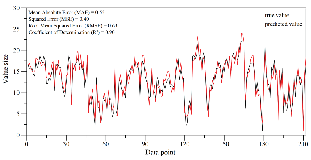
- Comparative analysis of LS-SVR predicted values and actual values, as well as test results.
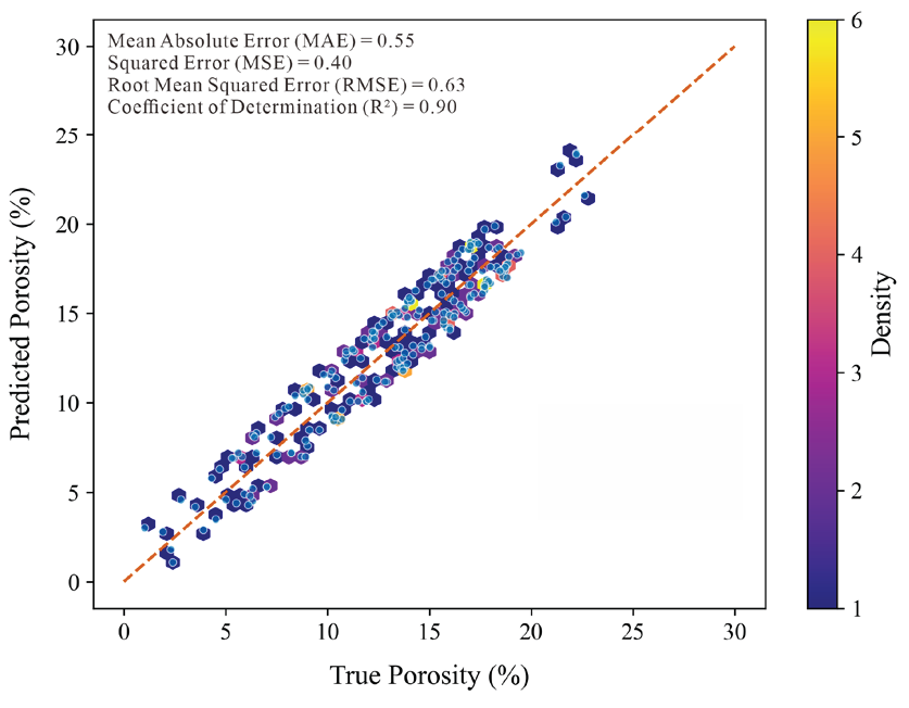
- Density scatter plot between the predicted porosity value of LS-SVR model and the actual porosity value (The horizontal axis (X axis) represents the true value (Φ), and the vertical axis (Y axis) represents the predicted value).
5.2 Discussion
In this study, the LS-SVR model was used to predict porosity based on selected geological and geophysical features. To assess the effectiveness of LS-SVR in a more intuitive manner, the MAE, MSE, RMSE, and R2 were utilized to evaluate the model's predictive capability and generalization ability. The calculation formula is as follows:
The evaluation metrics include MAE (0.55), MSE (0.40), RMSE (0.63), and R2 (0.90) (Table 1). The evaluation metrics show that the LS-SVR model accurately captures the relationship between input features and porosity, leading to precise predictions.
To enhance the visual representation of the prediction results, Resform was utilized to visualize the well-log curves. The predicted porosity results for Well 1 are compared with the porosity data obtained from core samples. Fig. 11 illustrates the comprehensive well log plot for Well 1, where the hollow circles represent the predicted results obtained through the optimized model, and red diamonds represent the porosity measured from core samples. The lithological features in the study area include gray-brown oil-bearing medium sandstone, gray-brown oil-bearing fine sandstone, and gray-brown oil-bearing medium sandstone. The depth range of the core samples is from 1122.01 m to 1239.10 m.

- (a-b) The LS-SVR model based on training shows the porosity prediction of Well 1 and compares the measured porosity of the core with the predicted porosity value. (The LS-SVR model predicts the porosity value in hollow circles, and the core measurement of the porosity value in red diamonds.) Φt: True porosity, Φp: Predicted porosity.
It can be observed that the predicted results closely match the actual values. By examining the two subplots, it is evident that the predicted porosity response varies across different lithological sections. This demonstrates the LS-SVR model's ability to quantify the relationship between porosity and well logging, capturing the diverse impacts of different well log values on rock properties. The model exhibits its applicability across different lithologies.
The LS-SVR model, while effective for porosity prediction, exhibits several methodological limitations that merit attention. Computational inefficiencies arise when processing large datasets, particularly in high-dimensional feature spaces typical of geophysical data, where the quadratic scaling of kernel matrix operations imposes significant training time requirements. Model performance is critically dependent on input feature quality and data integrity. Noise in logging curves, imbalanced sample distributions, and insufficient coverage of key lithological features collectively degrade predictive accuracy. Furthermore, the model’s assumption of static input-output relationships fails to capture the dynamic and nonlinear interactions observed in complex geological environments, such as those induced by diagenesis or tectonic stress. To address these challenges, future research should prioritize advanced feature selection methodologies, such as principal component analysis, which can reduce dimensionality and enhance feature representation. Integrating multi-source geophysical data through Bayesian optimization frameworks can improve model robustness against noise and variability. Incorporating detailed geological information, including stratigraphic and diagenetic constraints, may offer further insights into geological variability and refine predictive capabilities. Overall, the LS-SVR framework demonstrates robust prediction accuracy and stability, supporting its application in porosity estimation for geological exploration and oil and gas development. Comparative studies with alternative models, such as Gaussian process regression and deep neural networks, should evaluate performance across prediction accuracy, training efficiency, and model complexity to identify optimal solutions for specific geological scenarios.
6. Conclusions
-
1.
The LS-SVR model demonstrated strong predictive performance in porosity estimation, achieving an R2 of 0.90, MAE of 0.55, MSE of 0.40, and RMSE of 0.63. It significantly outperforms traditional empirical methods by utilizing well-logging and avoiding reliance on predefined formulas. Its capability to capture nonlinear relationships with porosity makes it especially suitable for large-scale, complex geological environments where traditional methods face limitations.
-
2.
While the LS-SVR model achieves high accuracy in porosity prediction, its performance depends on the quality and representativeness of the training data. In complex geological environments, the assumed stationary relationship between input features and porosity may not hold. Future research should focus on how to improve feature selection methods to improve the robustness of the model and respond to geological variability with more detailed geological information.
-
3.
The LS-SVR model's high predictive accuracy has significant practical implications, particularly for geological exploration and oil and gas development. Accurate porosity predictions guide reservoir characterization, well placement, and production optimization. This model offers a valuable tool for oil and gas professionals, improving decision-making in early reservoir development. Future work will address model limitations by exploring advanced techniques, such as multi-source data integration and machine learning model fusion, to further enhance prediction accuracy.
Acknowledgements
The authors express gratitude to all the reviewers who contributed to the review process, and to China National Petroleum Corporation Limited for which providing data and Resform software for use in this research. This research was supported by the Interpretative Processing and Reservoir Prediction Study for the 3D zone of Well No. 34400000-24-ZC0607-0061.
CRediT authorship contribution statement
Jingrui Chen: Conceptualization, Formal Analysis, Methodology, Software, Validation, Visualization, Writing – Original Draft, Writing – Review & Editing. Xin Chen: Formal Analysis, Methodology, Validation, Writing – Review & Editing. Ruizhao Yang: Funding Acquisition, Project Administration, Supervision, Writing – Review & Editing. Jianqi Lu: Formal Analysis, Methodology, Writing – Review & Editing. Tingting Li: Software, Project Administration, Supervision, Writing – Review & Editing.
Declaration of competing interest
The authors declare that they have no known competing financial interests or personal relationships that could have appeared to influence the work reported in this paper.
Data availability
The data that support the findings of this study are available from the corresponding author upon reasonable request.
Declaration of Generative AI and AI-assisted technologies in the writing process
The authors confirm that there was no use of artificial intelligence (AI)-assisted technology for assisting in the writing or editing of the manuscript and no images were manipulated using AI.
Funding
The Interpretative Processing and Reservoir Prediction Study for the 3D zone of Well No. 34400000-24-ZC0607-0061.
References
- Comparison of machine learning methods for estimating permeability and porosity of oil reservoirs via petro-physical logs. Petroleum. 2019;5:271-284.
- [CrossRef] [Google Scholar]
- Integration of multiple bayesian optimized machine learning techniques and conventional well logs for accurate prediction of porosity in carbonate reservoirs. Processes. 2023;11:1339. https://doi.org/10.3390/pr11051339
- [CrossRef] [Google Scholar]
- Ensemble machine learning: An untapped modeling paradigm for petroleum reservoir characterization. J. Pet. Sci. Eng.. 2017;151:480-487. https://doi.org/10.1016/j.petrol.2017.01.024
- [CrossRef] [Google Scholar]
- Reservoir rock permeability prediction using Svr based on radial basis function kernel. Carbonates and Evaporites. 2019;34:699-707.
- [CrossRef] [Google Scholar]
- Permeability determination of cores based on their apparent attributes in the persian gulf region using navie bayesian and random forest algorithms. J. Nat. Gas Sci. Eng.. 2017;37:52-68. https://doi.org/10.1016/j.jngse.2016.11.036
- [CrossRef] [Google Scholar]
- A rapid flood inundation model for hazard mapping based on least squares support vector machine regression. J. Flood Risk Management. 2019;12:e12522. http://dx.doi.org/10.1111/jfr3.12522
- [Google Scholar]
- A training algorithm for optimal margin classifiers. Proceedings of the fifth annual workshop on Computational learning theory 1992:144-152.
- [CrossRef] [Google Scholar]
- Measurement of Dependent Variables–Petrophysical Variables.
- Tectonic interpretation and geologicalmodeling of Deng-3 in S Block, Shuangcheng Area. Northeast Petroleum University; 2021.
- A multiscale and multivariable differentiated learning for carbon price forecasting. Energy Economics. 2024;131:107353. https://doi.org/10.1016/j.eneco.2024.107353
- [CrossRef] [Google Scholar]
- Machine learning and LSSVR model optimization for gasification process prediction. Multiscale and Multidiscip. Model. Exp. Des.. 2024;7:5991-6018. https://doi.org/10.1007/s41939-024-00552-x
- [CrossRef] [Google Scholar]
- Lithology identification using kernel fisher discriminant analysis with well logs. J. Pet. Sci. Eng.. 2016;143:95-102. https://doi.org/10.1016/j.petrol.2016.02.017
- [CrossRef] [Google Scholar]
- Speed up grid-search for parameter selection of support vector machines. Applied Soft Computing. 2019;80:202-210. https://doi.org/10.1016/j.asoc.2019.03.037
- [CrossRef] [Google Scholar]
- Multiple predicting K-fold cross-validation for model selection. J. Nonparametr. Stat.. 2017;30:197-215. https://doi.org/10.1080/10485252.2017.1404598
- [Google Scholar]
- Capability of self-organizing map neural network in geophysical log data classification: Case study from the Ccsd-Mh. J. Appl. Geophy.. 2015;118:37-46. http://dx.doi.org/10.1016/j.jappgeo.2015.04.004
- [Google Scholar]
- Is support vector regression method suitable for predicting rate of penetration? J. Pet. Sci. Eng.. 2020;194:107542 . http://dx.doi.org/10.1016/j.petrol.2020.107542
- [Google Scholar]
- Study on least squares support vector machine theory and its application. Lanzhou University. 2022;56
- [Google Scholar]
- Equipment and experimental methods for obtaining laboratory compression characteristics of reservoir rocks under various stress and pressure conditions. SPE Annual Technical Conference and Exhibition. 1977 SPE, SPE-6855-MS
- [Google Scholar]
- Integrated analysis of wireline logs analysis, seismic interpretation, and machine learning for reservoir characterisation: Insights from the late eocene mcKee formation, onshore taranaki basin, New zealand. J. King Saud Univ. Sci.. 2024;36:103221. https://doi.org/10.1016/j.jksus.2024.103221
- [CrossRef] [Google Scholar]
- Integration of spectral, spatial and morphometric data into lithological mapping: a comparison of different machine learning algorithms in the Kurdistan region. Ne Iraq. J. Asian Earth Sci. ;146:90-102. http://dx.doi.org/10.1016/j.jseaes.2017.05.005
- [CrossRef] [Google Scholar]
- Prediction of permeability and porosity from well log data using the nonparametric regression with multivariate analysis and neural network, Hassi R’mel Field, Algeria. Egypt. J. Pet.. 2017;26:763-778. https://doi.org/10.1016/j.ejpe.2016.10.013
- [Google Scholar]
- A new approach for porosity and permeability prediction from well logs using artificial neural network and curve fitting techniques: A case study of Niger delta, Nigeria. J. Appl. Geophy.. 2020;183:104207. https://doi.org/10.1016/j.jappgeo.2020.104207
- [CrossRef] [Google Scholar]
- Support vector method for function approximation, regression estimation, and signal processing, neural information processing systems. Vol vol 9. Cambridge: MIT Press; 1997.
- Prediction of triaxial mechanical properties of rocks based on mesoscopic finite element numerical simulation and multi-objective machine learning. J. King Saud Univ. Sci.. 2023a;35:102846. http://dx.doi.org/10.1016/j.jksus.2023.102846
- [Google Scholar]
- A novel method for petroleum and natural gas resource potential evaluation and prediction by support vector machines (Svm) Appl. Energy. 2023b;351:121836. https://doi.org/10.1016/j.apenergy.2023.121836
- [Google Scholar]
- Application of machine learning for evaluating and predicting fault seals: A case study in the huimin depression, Bohai Bay Basin, Eastern China. Geoenergy Sci. Eng.. 2023c;228:212064. https://doi.org/10.1016/j.geoen.2023.212064
- [Google Scholar]
- Ph.D. Dissertation, Department of Geology and Geophysics, Texas A&M University, College Station, Texas, United States, December 2004.
- A method to evaluate pore structures of fractured tight sandstone reservoirs using borehole electrical image logging. AAPG Bulletin. 2020;103:205-226. http://dx.doi.org/10.1306/04301917390
- [CrossRef] [Google Scholar]
- Evaluation of machine learning methods for formation lithology identification: a comparison of tuning processes and model performances. J. Pet. Sci. Eng.. 2017;160:182-193. https://doi.org/10.1016/j.petrol.2017.10.028
- [Google Scholar]
- Using machine learning methods to identify coal pay zones from drilling and logging-while-drilling (Lwd) data. SPE J.. 2020;25:1241-1258. http://dx.doi.org/10.2118/198288-PA
- [CrossRef] [Google Scholar]
- An efficient gradient-based model selection algorithm for multi-output least-squares support vector regression machines. Pattern Recognit. Lett.. 2018;111:16-22. https://doi.org/10.1016/j.patrec.2018.01.023
- [CrossRef] [Google Scholar]


