

Translate this page into:
Performance of logistic regression and support vector machine conjunction with the GIS and RS in the landslide susceptibility assessment: Case study in Nakhon Si Thammarat, southern Thailand
⁎Corresponding author. chedtaporn.su@wu.ac.th (Chedtaporn Sujitapan)
-
Received: ,
Accepted: ,
This article was originally published by Elsevier and was migrated to Scientific Scholar after the change of Publisher.
Abstract
The occurrence of landslides has risen in the past few decades, particularly in mountainous regions worldwide, including Nakhon Si Thammarat, southern Thailand. Despite various methods being employed for the initial management of landslide disasters, none have proven universally effective. The goal of this research is to create and assess landslide susceptibility maps (LSMs) within this area by employing support vector machine (SVM) and logistic regression, together with Geographic Information System (GIS) and Remote Sensing (RS) techniques. Eleven factors contributing to landslides were identified as topographic, environmental, and geological influences. The 365 landslides in the past were aimlessly selected into training (70%) and testing (30%) datasets. The four LSMs indicated that approximately 13%–20% of this study area exhibit a high susceptibility to landslides corresponding to the regions of high elevation with relatively steep slope angles. To evaluate and compare LSM models, the AUC value for training dataset were 0.977, 0.975, 0.958, and 0.967 and testing dataset were 0.973, 0.969, 0.956, and 0.964 for SVM with the radial basis function (rbf) kernel, SVM with polynomial deg 2, SVM with linear kernel and logistic regression models, respectively. Among these models, SVMs with rbf demonstrated the highest prediction rate. However, it requires a significant amount of time to choose the best parameters for achieving the highest accuracy prediction. In summary, these maps are applicable at the regional level to enhance the management of landslide hazards.
Keywords
Landslide susceptibility maps (LSMs)
Logistic regression
Support vector machine (SVM)
Geographic Information System (GIS)
AUC

1 Introduction
Landslides emerge as the most devastating natural disasters, resulting in significant impact on infrastructure, loss of lives, and disruption to communities worldwide (Zêzere et al., 2017; Froude and Petley, 2018). Nakhon Si Thammarat is a region in southern Thailand that frequently encounters risks of landslides due to the rugged mountainous and hilly terrain along with extremely heavy monsoon rainfall (Harper, 1993; Kanjanakul et al., 2016; Sujitapan et al., 2023). Moreover, the additional elements contributing to landslides in this region are geological setting, weathering characteristics, deforestation, and improper land utilization exacerbated by population expansion (Phien-Wej et al., 1993; Salee et al., 2022). The largest landslide event in this region occurred in November 1988 and was the most severe landslide recorded in Thailand’s history. These landslide events impacted the value of economic loss of more than 300 million US dollars and there were approximately 230 casualties (Tanavud et al., 2000; Komori et al., 2018). The Department of Mineral Resource (DMR) of Thailand has created a database of major landslides in the country since 1988, see Fig. 1. It discloses that the frequency of major landslides has been escalated in this area. With this growing occurrence and intensity of extreme weather events, it is crucial to create precise and dependable maps indicating the susceptibility to landslides for effective reformulating land utilization planning and strategies for mitigating risks in this region (Huang and Zhao, 2018).
Landslide susceptibility prediction plays a crucial role in assessing the likelihood of landslide occurrences across geographic areas and serves as a crucial technology for landslide risk management, early warning systems, and comprehensive assessments (Huang et al., 2022; Nanehkaran et al., 2023). Generally, there are three main methods for evaluating landslide susceptibility (Corominas et al., 2013): physical methods such as Stability Index Mapping (SINMAP) (Pack et al., 1999), knowledge-based methods such as data-driven methods like frequency ratio (FR) (Shahabi et al., 2014, 2015), and analytical hierarchy process (AHP) (Mondal and Maiti, 2013; Zhang et al., 2016). A consensus regarding the most effective method for assessing landslide susceptibility remains elusive. However, it is widely acknowledged that data-based methods tend to be better suited for the landslide evaluation at a regional level (Corominas et al., 2013).
Over the past few years, methods involving Geographic Information System (GIS) and Remote Sensing (RS) have been employed together with data-based methods and machine learning algorithms, such as logistic regression and support vector machine (SVM). Both algorithms have gained popularity in landslide susceptibility mapping (Kalantar et al., 2017; Oh et al., 2018; Chen et al., 2018; Nhu et al., 2020; Nikoobakht et al., 2022). Based on the presumption that forthcoming landslides are likely to occur under similar conditions as past landslide occurrences, the data-based methods with machine learning employ scientific models to forecast the feasibility of landslide events (Meng et al., 2024). These models utilize the spatial distribution of various factors influencing landslides within the susceptible areas (Reichenbach et al., 2018). The utilization of logistic regression and SVM algorithms offers distinct advantages in landslide susceptibility mapping (Azarafza et al., 2021).
Logistic regression allows for the identification and quantification of the relative significance of various landslide-related factors, aiding in the identification of critical variables and their influence on landslide susceptibility (Bai et al., 2010; Nolasco-Javier and Kumar, 2021). As many factors may affect landslide occurrences, implementing a hypothesis test on the logistic regression is one way to identify a related factor. It is a rigid supervised machine learning model. The support vector machine is a powerful machine learning algorithm that seeks to identify an optimal hyperplane for separating landslide and non-landslide areas in a multidimensional feature space (Arora et al., 2004; Lee et al., 2017). SVM excels in managing intricate data patterns and non-linear correlations between input variables, making it a valuable tool for landslide susceptibility mapping (Chang et al., 2023). By capturing the underlying patterns and classifying areas into different susceptibility levels, SVM can contribute to accurate and reliable mapping results (Huang and Zhao, 2018). The SVM is one of the flexible supervised machine learning models.
The objective of this study is to evaluate and compare the performance of logistic regression and SVM in generating landslide susceptibility maps. By utilizing these algorithms, we seek to improve our understanding of the spatial distribution and factors influencing landslide occurrences in Nakhon Si Thammarat, where has witnessed recurrent landslide events, making it a suitable candidate for this research. Here, we collected a comprehensive dataset that includes information on slope, elevation, lithology, land cover, and rainfall, among other relevant variables. These variables were chosen due to their recognized impact on the incidence of landslides. The dataset was separated into training and validation sets, utilizing for the development and evaluation of both logistic regression and SVM models.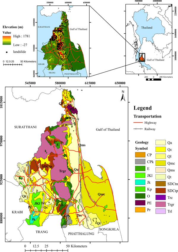
Geological map (below) and 30 m-DEM (top) of Nakhon Si Thammarat province with landslide events (black circle).
By comparing the performance of these models using appropriate evaluation methods, we aim to determine their effectiveness in landslide susceptibility mapping and identify their strengths and limitations. Decision-makers, land-use planners, and other stakeholders involved in disaster risk management will find great value in this study’s findings. The resulting landslide susceptibility maps can aid in identifying high-risk areas, prioritizing mitigation measures, and improving emergency preparedness efforts. Moreover, the comparative analysis of logistic regression and SVM will contribute to the existing body of knowledge on machine learning techniques for landslide susceptibility mapping, facilitating the adoption of appropriate methodologies in similar contexts.
In the subsequent segments of this paper, we present the description of the study area, the methodology employed for data collection, preprocessing, and modeling using logistic regression and SVM. Subsequently, we discuss the results and comparative performance of the two algorithms, followed by a comprehensive discussion of the findings. Finally, we summarize the key findings and their practical implications.
2 Description of research area
The research area is Nakhon Si Thammarat province situated in the south of Thailand, rests along the eastern coast of the Thai Peninsula (Fig. 1) (Pramojanee et al., 1998). There are three main land-scarps in this province: the mountain range, namely Khao Luang and low hills in the middle; the intermountain upland or intermediate zone connecting a mountain range to a plain or lowland at the southwest; and the coastal plain at the east.
In the Khao Luang mountain range, the highest peak of elevation is approximately 1800 m above mean sea level (Fig. 1) (Pramojanee et al., 1998) and the slopes are fairly steep with average angles of about 27–33 degrees. The bedrock geology in the mountain range (Ridd et al., 2011) is coarse-grained granite to granite gneiss of Triassic to Cretaceous age (light pink area marked ‘Trgr’ in Fig. 1). Older metamorphic and sedimentary rocks are located in low-hill areas. They are quartzite and sandstone of Precambrian age (light green area marked ‘E’ in Fig. 1), brown shale and siltstone of Silurian to Carboniferous age (dark brown area marked ‘SDCtp’ in Fig. 1), Ordovician limestone (dark green area marked ‘O’ in Fig. 1), and pebbly mudstone and gray shale of Carboniferous to Permian age (gray area marked ‘CPk’ in Fig. 1). To the west of the mountain range are scattered with low hills and intermountain upland at an average elevation of 100–120 m. The bedrock geology of low hills consists of argillaceous limestone interbedded with shale of Jurassic age (medium apple green area marked ‘Jk’ in Fig. 1) and arkosic sandstone of Jurassic to Cretaceous age (tourmaline green area marked ‘JKl’ in Fig. 1). The intermountain upland is veiled by colluvial and terrace sediments in Quaternary age (yellow areas marked ‘Qc’ and ‘Qt’ in Fig. 1). To the eastern side of the mountain range lies a gently undulating piedmont plain, which gradually descends eastward from the foothills of the range to the coastal plain and the sea. On average, the distance between the foothills and the sea is approximately 30 km, with the foothills standing at an elevation averaging 150 meters above sea level, while the shore is at about 2 meters above sea level (Pramojanee et al., 1998). Therefore, the slope gradient from the foothills of the mountain range to the sea is notably steep. Moreover, numerous small streams and rivers are present on either side of the range. This eastern area is mainly covered by alluvial and coastal tide-dominated sediments in the Quaternary age (yellow areas marked ‘Qa’ and ‘Qmc’ in Fig. 1).
In addition to geography and geology, this province is in an area of intense rainfall (Pal et al., 2018). According to Kottek et al. (2006) climate classification, this province has a climate characterized by Tropical Monsoon conditions with annual precipitation intensity fluctuating between 1800 and 2200 mm, which is susceptible to triggering landslides (Schmidt-Thomé et al., 2018). The beginning of the rainy season typically occurs in mid-May and extends through to mid-January. The highest monthly rainfall intensity exceeding 200 mm usually falls in October and November, accompanied by frequent rainstorms (Loo et al., 2015). The summer season consists of March and April. The average temperature and relative humidity of the province are 27 Celsius and 78 percent respectively (Pramojanee et al., 1998).
According to this Tropical Monsoon climate together with geography and geology in this province, the regional characteristics of landslides may differ from other areas. Many landslides have emerged in the topsoil, which is typically composed of residual soils (Rahimi et al., 2010; Sujitapan et al., 2023). The characteristic of these landslides is shallow landslide with debris flow from Cruden (1996) classification. The residual soils have resulted from the granitic rock weathering process that contains silty sand and sandy silt with occasional gravel traces. Rainfall-triggered slope failures predominantly happen in the unsaturated vadose zone above the groundwater table of the residual soils (Rahardjo et al., 2012). As rainfall seeps into the soil pores, it elevates the soil’s moisture level, causing a decrease in matric suction and shear resistance within the unsaturated soil. As a consequence, the slope becomes more prone to failure (Tan et al., 2021). Moreover, human activities like urbanization, deforestation, mining, construction, and inadequate land management practices are able to significantly influence landslide occurrence in this province. Activities that alter natural drainage patterns or destabilize slopes can also exacerbate landslide hazards (Sujitapan et al., 2024).
3 Materials and methods
There are two steps of the methodology: (i) data preparation, and (ii) landslide susceptibility analysis. The flowchart implemented in this study is revealed in Fig. 2. In the data preparation, a landslide inventory map and influencing factors of landslides were obtained by GIS and RS to understand the relation between the past landslides and the influencing factors of landslides. Subsequently, the landslide susceptibility is assessed using logistic regression and SVM. More details are described below.
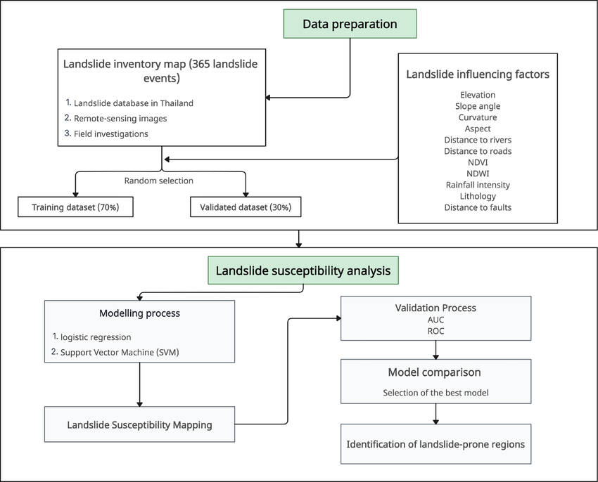
Methodology flowchart in this study.
3.1 Landslide inventory map
The landslide inventory map reveals the locations of existing landslides, see Fig. 1. It has been produced by the landslide database in Thailand from 1989 to 2022, interpretation from remote-sensing images, and field investigations. All 365 landslides were identified in this area. They were converted to 8025 landslide pixels of 30 × 30 m each. These landslide pixels were subsequently merged with 2772 pixels of 30 × 30 m each representing areas without landslides, which were chosen randomly from regions unaffected by landslides. The total count of landslide and non-landslide pixels was separated into train and test datasets. After the landslide susceptibility models were created using the training dataset, the testing dataset was utilized to evaluate and validate the models’ effectiveness.
3.2 Landslide influencing factors
Here, the picking of triggering factors is critical for understanding the underlying mechanisms and drivers of landslide occurrence. These triggering factors are chosen based on their known influence on slope stability and their relevance to the specific geological, topographical, and climatic conditions of the study area. Therefore, eleven influencing landslide factors shown in Fig. 3 are chosen according to findings from prior research, such as Phien-Wej et al. (1993), Tanavud et al. (2000), Kanjanakul et al. (2016), and Sujitapan et al. (2023) of the characteristics and mechanism of landslide occurrences in this area. They can be divided to three categories: topographical, environmental, and geological groups (Chen et al., 2018). The topographical factors comprise elevation, slope angle, curvature, aspect, distance to rivers, and distance to roads. Normalized Difference Vegetation Index (NDVI), Normalized Difference Water Index (NDWI), and rainfall are determined as environmental factors, while lithology and distance to faults are geological factors. The details of the eleven factors are explained below and summarized in Table 1.
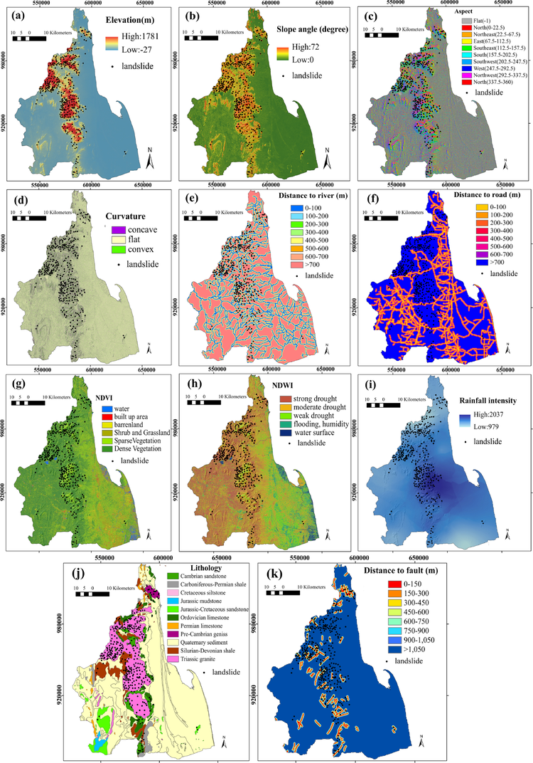
Map of eleven influencing landslide factors: (a) elevation; (b) slope angle; (c) aspect; (d) curvature; (e) distance to rivers; (f) distance to roads; (g) NDVI; (h) NDWI; (i) rainfall intensity; (j) lithology; and (k) distance to faults.
3.2.1 Elevation
An elevation map was derived from Digital Elevation Model (DEM) data, featuring a spatial resolution of 30 × 30 meters in this study area. This DEM was generated by Shuttle Radar Topography Mission (SRTM) dataset obtained from the USGS Earth Explorer website. This factor stands out as one of the most influential topographic factors contributing to slope failure in this area (Tanavud et al., 2000). The elevation map within this area spans from −27 to 1781 m above sea level (Fig. 3a).
3.2.2 Slope angle
The slope angle expresses the changes in elevations over distance. It affects the level of soil moisture concentration and water flows in the subsurface, directly related to landslide occurrences. A slope angle map of this area was generated from the DEM data using spatial analyst tools in ArcGIS 10.5 software. In this area, the frequency of landslides is likely to occur in the steep slope (Tanavud et al., 2000). The slope angle map is in the range of 0 to 72 degrees (Fig. 3b).
3.2.3 Aspect
The aspect denotes the bearings of the slope face measured in the clockwise direction from 0 to 360 degrees. It relates to directions of precipitation, wind, and sunlight exposure. This can control the growth of vegetation, rate of erosion, and thickness of soil resulting in landslide occurrence. An aspect map of this area was created from the DEM data as a slope angle. It is classified into ten directions of Flat, North, Northeast, East, Southeast, South, Southwest, West, Northwest, and North (Fig. 3c).
3.2.4 Curvature
The curvature displays the shape of the slope which can probably affect the landslide occurrence. An aspect map of this area was also created from the DEM data. It can be divided into three classes: concave ( −0.05), flat (−0.05 to 0.05), and convex ( 0.05) (Fig. 3d). The probability of landslide occurrence is higher in concave and convex areas compared to flat areas.
3.2.5 Distance to rivers
The stability of slopes is significantly influenced by the familiarity of these slopes to the river networks (Alexakis et al., 2013). Many landslides in this area have occurred close to river networks. The river networks in this study area were derived from the topographic map at a scale of 1: 50000 obtained from Department of Mineral Resources (DMR), Thailand. A distance to rivers map of this area was calculated and generated by the Euclidean Distance Tool in ArcGIS 10.5 software. The distances are classified into eight intervals: 0–100, 100–200, 200–300, 300–400, 400–500, 500–600, 600–700, and m (Fig. 3e).
3.2.6 Distance to roads
The building roads near the mountain significantly influence the landslide distribution in this area. In the vicinity of road networks, widespread excavation, additional loads, and deforestation are frequently noted, contributing to the susceptibility of slope failures. The road networks in this area were also derived from the topographic map at the same scale as distance to rivers. A distance to roads of this area (Fig. 3f) was generated by the Euclidean Distance Tool and classified into eight intervals as same as the distance to rivers map.
3.2.7 NDVI
NDVI is the assessment of vegetation growth and the distribution of soil characteristics through the analysis of spectral changes in green vegetation (Sonker et al., 2022). An NDVI map of this study area (Fig. 3g) was generated from red and near-infrared bands of Landsat 8 OLI satellite images together with ArcGIS 10.5 software. The NDVI map is classified into six categories (water, built-up areas, barren land, shrub and grassland, sparse vegetation, and dense vegetation) according to NDVI values.
3.2.8 NDWI
NDWI is used to detect the presence of moisture content. High NDWI values indicate the existence of elevated moisture levels (Ullah et al., 2022). An NDWI map of this study area (Fig. 3h) was derived from green and infrared bands of Landsat 8 OLI satellite images together with ArcGIS 10.5 software. The NDWI values are divided into five classes: water surface, flooding or humidity, weak drought, moderate drought, and strong drought.
3.2.9 Rainfall intensity
Rainfall is an external variable frequently employed in landslide susceptibility analysis (Moazzam et al., 2020). The annual rainfall intensity is normally high, which is susceptible to triggering landslides (Sujitapan et al., 2023). The rainfall intensity data was acquired from the 9 year average annual rainfall intensity of sixty-seven stations in this study area measured by Thailand Royal Irrigation Department. A rainfall intensity map of this study area (Fig. 3i) was then generated by interpolation through the kriging method in ArcGIS 10.5 software. The rainfall intensity value is in the range of 979 to 2037 mm.
3.2.10 Lithology
Lithological types exhibit unique strength and slope structures, significantly influencing the landslides. The landslides in this study area frequently occur in the granitic bedrock, which is a high rate of weathering (Tanavud et al., 2000). A lithological map of this area (Fig. 3j) was achieved from the geological map (Fig. 1) at a scale of 1:100,000 from the DMR. The lithology is separated into eleven kinds based on the type of bedrock and age.
3.2.11 Distance to faults
Faults are tectonic fractures that weaken rock strength and typically result in extensive fracturing and precarious slope conditions (Pourghasemi and Rahmati, 2018). Consequently, they can significantly increase landslide occurrence. The faults in this study area were extracted from a geological structure map with a scale of 1: 50000 obtained from DMR. A distance to faults map of this area was created by the Euclidean Distance Tool and classified into eight intervals: 0–150, 150–300, 300–450, 450–600, 600–750, 750–900, 900–1050, and 1050 m (Fig. 3k).
However, integrating influencing factors into landslide susceptibility models (LSM) in Nakhon Si Thammarat can indeed present several challenges, especially concerning data availability and quality. One of the primary challenges is the availability of reliable data for the various triggering factors. In some cases, data may be limited or unavailable for certain parameters such as soil properties, geological characteristics, or historical landslide events. This scarcity can hinder the development and validation of LSM models. Even when data is available, its quality may vary. Incomplete, outdated, or inaccurate data can compromise the accuracy and reliability of LSM models. Ensuring data quality through rigorous validation, verification, and quality control measures is essential for robust landslide susceptibility assessment.
Factors
Data source
Scale
Year of
acquisition
Elevation
DEM from USGS
30 × 30 m
2017
Slope angle
Aspect
Curvature
Distance to rivers
Shapefile from DMR
1: 50000
2012
Distance to roads
Distance to faults
Lithology
NDVI and NDWI
LandSat8 images from USGS
30 × 30 m
2022
Rainfall intensity
Rainfall data from Thailand
30 × 30 m
Avg. from
Royal Irrigation Department
2015–2023
3.3 Machine learning algorithms for modeling approach
Here, the logistic regression and SVM are used for landslide susceptibility mapping. They offer different approaches to identifying and predicting areas at risk of landslides based on available data and input factors. In this section, we first verify which factor discussed above has a statistical effect on the landslide occurrence by using a hypothesis test on the logistic regression model. The hypothesis test shows the P-values for each considered factor in which we can eliminate the uncorrelated factors. The results show that rainfall intensity, aspect, and NDWI data do not affect the landslide occurrence. We can now consider the 8 remaining factors affecting landslide susceptibility: elevation, slope angle, curvature, distance to rivers, distance to roads, NDVI, lithology, and distance to faults.
3.3.1 Logistic regression
Here, the binary outcome, a landslide or a non-landslide, is modeled using logistic regression. Assume that we have
data written in the form
for
and
where
is a vector of predictors and
is the response value related to
. For each
, the vector
consists of 136 elements; 7 relevant quantitative factors discussed above and 129 dummy variables from the qualitative factor of lithology. The predictor
then can be written in the form
where
. The response
falls into one of two categories, landslide (
) and non-landslide (
). Given that
is the conditional probability, the logistic regression used in this manuscript is a statistical model presenting a relationship between
and
as follows:
3.3.2 Support vector machine
Support vector machines (SVMs) are among the most important machine-learning tools to classify data where is a vector of predictors and is the binary response of 1 (landslide) or −1 (non-landslide). SVM’s primary goal is to create the best-separating hyperplane possible for categorizing the landslide data that has been collected.
Now suppose that we have
data of predictors and responses, say
for
where
and each predictor
consists of
factors; i.e.,
. Define a
dimensional hyperplane as
, which is equivalent to the vector form equation:
-
is called linear kernel,
-
is called radial basis function kernel,
-
is called polynomial kernel.
3.3.3 Model performance comparison
The model performance based on the considered methods (Logistic regression and SVM) has been investigated by considering sensitivity value, specificity value, accuracy value, ROC & AUC, and -fold cross-validation.
Sensitivity describes how effectively a model can identify pixels representing landslides as indicative of landslides. The sensitivity value is calculated by where FN value is the number of pixels that are truly landslides but were mistakenly categorized as non-landslides by the model, and TP value indicates the number of landslide pixels that are accurately identified as landslides.
Specificity quantifies the percentage of real, non-landslide pixels that a model accurately identifies. The specificity value is calculated by where TN denotes the number of pixels the model correctly labels as non-landslides and FP denotes the number of pixels the model wrongly labels as landslides when they are actually non-landslides.
We note here that the higher of both sensitivity and specificity values the better performance of the model. In the landslide situation, the model with the higher sensitivity value would have better performance in the sense that it can predict the landslide pixels correctly as landslides. The general comparison of the model performances is observed by computing,
A helpful tool for assessing the trade-off between the TP rate (sensitivity) and the FP rate (1-specificity) at various classification thresholds is the ROC curve. The threshold used in the logistic model is the probability value and the one implemented in the support vector machine is the decision value.
Another method for assessing the performance of a model is called K-fold cross-validation. The whole dataset is separated into groups, or folds. In total of times trained model, each time a new fold is considered as testing and the remaining folds are the training dataset. In this manuscript, we consider the case of . Since this process produces the accuracy in each running time, the general accuracy of the model is the average of the 10 accuracies.
3.3.4 Generating landslide maps
This subsection is devoted to illustrating how the predicted landslide map (Fig. 4) of each model is created. It is obvious from the logistic regression model that it produces a probability for a given input predictor. The predicted landslide map using this model is directed from the values of the predicted probabilities. The support vector machine; on the other hand, produces the value of the hyperplane function at a considered predictor. This value is not the probability of landslide occurrence. To achieve the probability value for each landslide predictor, we consider the sigmoid function: where is a vector of landslide predictor and is the hyperplane function obtained from the SVM method. These sigmoid values are considered as the probability values used to generate the landslide prediction maps.
4 Results and discussion
4.1 Landslide susceptibility map evaluation
The landslide susceptibility maps with probability value (0–1) are shown in Fig. 4. In the maps, each pixel size 30 × 30 meters is categorized into five classes: very low (0–0.13), low (0.13–0.33), medium (0.33–0.58), high (0.58–0.83), and very high (0.83–1.00) using the natural break method. Fig. 4(a) is the map created by the method of logistic regression. The maps generated by the support vector machine with the linear kernel (LR), the radial basis function (rbf) kernel, and the polynomial kernel are shown in Fig. 4 panels (b), (c), and (d), respectively. These generated landslide susceptibility maps adhere to two spatial effectiveness criteria when utilizing the four models: (1) the high-susceptibility category encompasses only mountainous regions, and (2) the most of landslide pixels are present in this category. Fig. 4 is consistent with the elevation map of this area (Fig. 3a) that regions with high elevation are susceptible to landslides, while low-elevation areas, such as river basins and coastal plains characterized by low elevation and flat terrain, are devoid of landslide occurrences. This pattern of landslide distribution highlights the susceptibility of hilly areas to landslides, as manifested in the susceptibility map.
Furthermore, the proportion of susceptible zones included by all models are also revealed in Fig. 5. The results show that all models cover over 55% of the area with a very low susceptible zone, which constitutes a majority of the entire study area. All SVM models exhibit very high susceptible zones of 17%–20%. In contrast, they categorize the low to high susceptible zones homogeneously with the areas of 5%–10%. The very high susceptible zone of the logistic regression model covers 13% of the total area which is a comparatively smaller portion than the SVM models. However, the rationality of the Landslide Susceptibility Model (LSM) was also assessed by frequency ratio (fr), which is the proportion of the number of landslides within each susceptibility class. All models exhibited a consistent pattern, demonstrating a higher concentration of landslides in the highly susceptible zones and fewer occurrences in low-lying regions (Fig. 4). The highest frequency ratio of landslides relating to the very high susceptible zone is SVM with the rbf kernel model (fr
4.44) followed by SVM with the polynomial kernel (fr
4.43), logistic regression (fr
4.39), and SVM with the linear kernel (fr
4.30).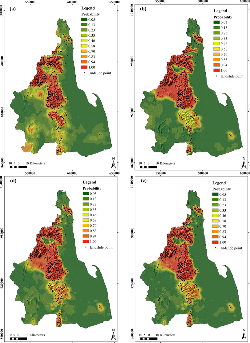
Landslide susceptibility maps generated by each model: (a) logistic regression; (b) SVM with the linear kernel; (c) SVM with the rbf kernel; and (d) SVM with the polynomial kernel.
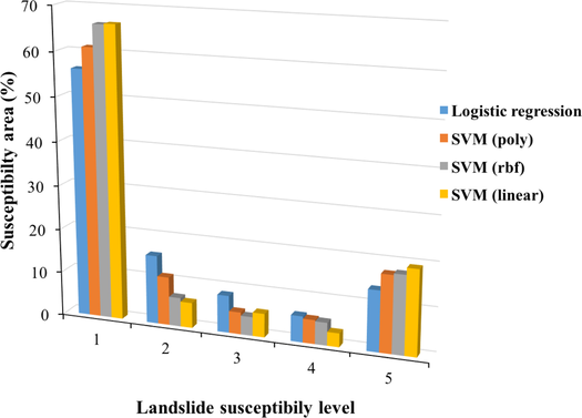
Percentages of each landslide susceptibility level in all models.
4.2 Accuracy of the maps and model comparison
To compare the accuracy of each model, the training dataset and the testing dataset used in each model need to be the same. In the computation process, we divided the whole dataset into 70% training and 30% testing. We then use the same division to analyze the performance of each model. The performance analysis of the models is present in Table 2. As presented in the support vector machine section, to solve the optimization problem (10) we need to specify the kernel and the fixed value of the tuning parameter . The values of and the tuning parameter shown in Table 2 have been collected as the best-fitted parameters for each model in the sense that those values produce the highest accuracy on the 70% training dataset. We note here that the process of choosing the best parameters is time-consuming. In the process, we choose and that produce the highest accuracy. For larger datasets, the data reduction method can reduce the computer running time. The basic idea of this method is to use a sufficient amount of data for training instead of using all training data to construct the hyperplane. For the SVM with linear kernel, , the best value of is . In the SVM with the radial basis function kernel, , the best-fitted values of and for the training dataset are 30 and 1 respectively, listed in Table 2. The SVM with the polynomial kernel, , degrees , , and have the best-fitted parameters and , and , and and , respectively, shown in Table 2.
In terms of the accuracy prediction on the training dataset, the SVM with the polynomial kernel deg 4 performs the best accuracy of 97.03%, followed by the SVM with polynomial deg 3 (96.53%), the SVM with polynomial deg 2 (96.14%), the SVM with the rbf kernel (96.01%), the SVM with the linear kernel (95.09%), and the lowest accuracy prediction is the logistic regression model (93.83%), see Table 2. Note that the higher accuracy of models on the training data does not imply the high performance of the model because overfitting may occur.
Models
Data
Actual
Actual
Specificity
Sensitivity
Accuracy
non-landslide
landslide
(%)
(%)
(%)
SVM
Train
Predicted non-landslide
1681
232
96.50
95.98
96.10
(rbf)
Predicted landslide
61
5541
Test
Predicted non-landslide
705
113
93.87
95.42
95.06
Predicted landslide
46
2357
SVM
Train
Predicted non-landslide
1720
193
98.29
96.65
97.03
(poly deg 4)
Predicted landslide
30
5572
Test
Predicted non-landslide
702
116
92.49
95.29
94.63
Predicted landslide
57
2346
SVM
Train
Predicted non-landslide
1693
220
97.64
96.19
96.53
(poly deg 3)
Predicted landslide
41
5561
Test
Predicted non-landslide
695
123
93.92
95.04
94.78
Predicted landslide
45
2358
SVM
Train
Predicted non-landslide
1684
229
96.50
96.03
96.14
(poly deg 2)
Predicted landslide
61
5541
Test
Predicted non-landslide
711
107
93.31
95.65
95.09
Predicted landslide
51
2352
SVM
Train
Predicted non-landslide
1603
310
96.45
94.70
95.09
(linear)
Predicted landslide
59
5543
Test
Predicted non-landslide
670
148
95.17
94.12
94.35
Predicted landslide
34
2369
Logistic
Train
Predicted non-landslide
1665
248
88.52
95.60
93.83
regression
Predicted landslide
216
5386
Test
Predicted non-landslide
699
119
86.62
95.07
92.95
Predicted landslide
108
2295
For the testing dataset, the accuracy predictions of the SVM with the polynomial kernel deg 2 and the SVM with the rbf kernel outperform the others with 95.09% and 95.06% accuracies, respectively. They are followed by the SVM with polynomial deg 3 (94.78%), the SVM with polynomial deg 4 (94.63%), the SVM with linear kernel (94.35%), and the logistic regression model (92.95%), see Table 2. This result can be a reason to conclude that the SVM with the polynomial kernel deg 2 and the SVM with the rbf kernel are the outperforming models.
The 10-fold cross-validation tests show that the SVM the polynomial kernel deg 3 produces the highest accuracy at 95.72% followed by the SVM with the polynomial kernel deg 4 (95.67%), the SVM with the rbf kernel (95.46%), the SVM with the polynomial kernel deg 2 (95.45%), the SVM(linear) (94.68%), and the logistic regression model (93.35%), see Table 3. The conducted cross-validation shows that the model performances slightly change when we randomly split the whole dataset into another 70% training and 30% testing.
Models
Average of accuracy
Standard deviation of accuracy
(%)
(%)
SVM(rbf)
95.46
0.601
SVM(poly deg 4)
95.67
0.499
SVM(poly deg 3)
95.72
0.577
SVM(poly deg 2)
95.45
0.681
SVM(linear)
94.68
0.782
Logistic regression
93.55
0.748
The ROC curve and the AUC value of each model shown in Fig. 6 confirm that the SVM with the rbf kernel outperforms the others for both training and testing datasets. For the training dataset, it reaches 0.97734 of AUC followed by the SVM with the polynomial degree 2 (AUC 0.97499), the SVM with the linear kernel (AUC 0.95754), and the logistic regression model (AUC 0.96683). For the testing dataset, the SVM with the rbf kernel shows 0.97313 of AUC followed by the SVM with the polynomial degree 2 (AUC 0.96904), the SVM with the linear kernel (AUC 0.95628), and the logistic regression model (AUC 0.96403). As a point on the ROC curve is the ordered pair of true positive rate and false positive rate values for a given cut point (decision value in the SVM case or probability value in the logistic regression case), a model with the AUC closer to 1 is a better model in general since it implies that there is a cut point which gives the highest value of the true positive rate and the lowest value of the false positive rate. This reason leads us to conclude that the SVM with the rbf kernel is the best method in general for generating a landslide susceptibility map.
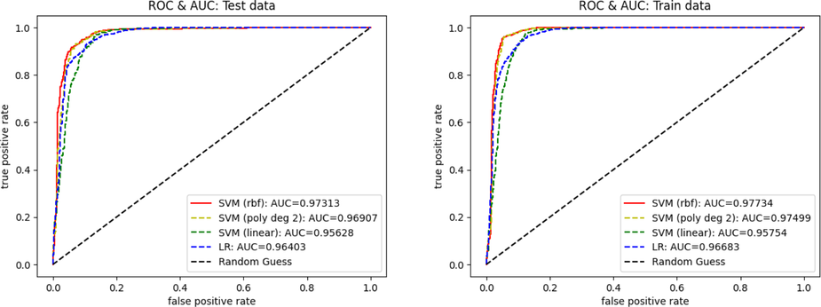
ROC curves for Test and Train data. The SVM with polynomial kernel deg 2 produces the highest AUC compared to other polynomial degrees.
4.3 Identification of landslide-prone regions in the study area
According to all landslide susceptibility maps, elevation and slope are the most contributing factors of landslides in this province. Both factors highlight that more than 60% of landslide events had occurred in Khao Luang mountain and low hills in the middle of this province (elevation more than 300 m) with relatively high slope angle (more than 30 degrees). Consequently, these regions are highly susceptible to landslides, corresponded to field observations. Moreover, the lithological factor is also important in triggering landslides. Most of the landslides (more than 70%) were present in the granitic rock of Triassic to Cretaceous age (light pink area in Fig. 1) due to high weathering and erosion in this type of rock. Although the river basin areas in the east part of this province are susceptible to erosion because of their low elevation and destructive forces, they do not qualify as landslide-prone areas.
However, the rise in landslide occurrences in mountainous regions can be linked to a blend of environmental and anthropogenic factors. The heavy rainfall, particularly during the monsoon season can saturate the soil and increase slope instability, leading to landslides. The mountainous terrain is inherently prone to landslides due to steep slopes, fragile geological formations, and tectonic activities. Deforestation and Land Use Changes, such as deforestation, urbanization, and infrastructure development can disturb the natural balance of ecosystems and increase landslide risk. Deforestation, in particular, reduces vegetation cover, which plays a crucial role in stabilizing slopes and preventing soil erosion. Rapid urbanization and unregulated land development practices in Nakhon Si Thammarat may exacerbate landslide hazards by altering drainage patterns, destabilizing slopes, and increasing surface runoff. Improper land use planning and construction on vulnerable slopes can escalate landslide risks. The construction of roads, highways, and other infrastructure projects in mountainous areas can disrupt natural slopes, leading to slope failures and landslides. Poorly designed or maintained infrastructure may exacerbate landslide incidents in Nakhon Si Thammarat. Population growth in mountainous regions of Nakhon Si Thammarat increases human exposure to landslide hazards. Settlements located in landslide-prone areas are particularly vulnerable, especially if adequate disaster preparedness measures are lacking.
Over time, the evolution of these factors, coupled with changing environmental conditions and human activities, has contributed to the escalating trend of landslide incidents in Nakhon Si Thammarat. Understanding these dynamics is crucial for implementing effective risk reduction strategies, land use planning policies, and sustainable development practices to reduce the effect of landslides on communities and the environment.
4.4 Integrating landslide susceptibility models to existing risk management
The landslide susceptibility models (LSMs) generated for Nakhon Si Thammarat can be integrated into existing risk management frameworks or utilized by various stakeholders, such as government agencies or local communities. Government agencies can use the LSMs to point out highly susceptible areas prone to landslides and integrating this data into land use planning processes. Zoning regulations and development restrictions can be implemented to avoid construction in landslide-prone zones. LSMs can also inform decisions regarding the planning, building, and upkeep of infrastructure projects like roads, bridges, and buildings. Government agencies can prioritize investments in landslide mitigation measures for critical infrastructure assets located in high-risk areas.
Furthermore, LSMs can raise awareness among local communities about landslide hazards and the factors contributing to susceptibility. Educational programs and community workshops can empower residents to adopt proactive measures to mitigate risks, such as slope stabilization techniques and evacuation plans. Local communities can collaborate with government agencies and NGOs to implement community-based adaptation measures based on LSM findings. This may include reforestation efforts, watershed management initiatives, and the establishment of early warning systems at the grassroots level. By integrating LSMs into existing risk management frameworks and engaging relevant stakeholders, Nakhon Si Thammarat can enhance its resilience to landslide hazards and mitigate the socio-economic impacts of landslide events effectively.
5 Conclusion
The results confirm that both logistic regression and SVM models are effective for predicting landslide susceptibility with over 93% accuracy. The selected factors are based on literature reviews and hypothesis testing. While SVM, especially with the rbf kernel, generally outperforms logistic regression in accuracy, 10-fold cross-validation, and AUC values, the difference in accuracy is less than 2%. Logistic regression offers the advantage of hypothesis testing to understand factor–response relationships. Among the SVM with different kernels, the SVM with the rbf kernel performs better in many aspects. It shows the highest frequency ratio, the highest accuracy prediction on both testing and training datasets, and the highest AUC value. However, the SVM requires time-consuming parameter tuning for optimal accuracy, because the parameters and need to be identified before solving the quadratic optimization to achieve the SVM model with rbf kernel and the additional identified degree for the polynomial kernel. The Python codes of the tuning processes are shown in the supporting information section.
The insights from landslide susceptibility assessments in this region can benefit other areas with similar challenges, such as Suratthani province. Understanding the unique triggering factors in different regions is crucial. Lessons learned here can help identify common triggers, like heavy rainfall, geological instability, land use changes, and human activities, applicable to other areas. Validated LSMs support land use planning, infrastructure development, and disaster risk management. Government agencies and stakeholders can use LSM outputs to prioritize interventions, implement preventive measures, and enhance preparedness. Further research should improve LSM accuracy by incorporating additional data, exploring alternative modeling techniques, and validating under various conditions. Integrating stakeholder feedback, field data, and robust validation will enhance the accuracy, reliability, and relevance of LSMs for landslide risk assessment and management.
CRediT authorship contribution statement
Kiattisak Prathom: Writing – original draft, Software, Methodology, Data curation, Conceptualization. Chedtaporn Sujitapan: Writing – original draft, Visualization, Validation, Conceptualization.
Declaration of competing interest
The authors declare that they have no known competing financial interests or personal relationships that could have appeared to influence the work reported in this paper.
References
- Integrated use of GIS and remote sensing for monitoring landslides in transportation pavements: The case study of paphos area in Cyprus. Nat. Hazards. 2013;72:119-141.
- [CrossRef] [Google Scholar]
- An artificial neural network approach for landslide hazard zonation in the Bhagirathi (Ganga) Valley, Himalayas. Int. J. Remote Sens.. 2004;25:559-572.
- [CrossRef] [Google Scholar]
- Deep learning-based landslide susceptibility mapping. Sci. Rep.. 2021;11
- [CrossRef] [Google Scholar]
- GIS-based logistic regression for landslide susceptibility mapping of the Zhongxian segment in the Three Gorges area, China. Geomorphology. 2010;115:23-31.
- [CrossRef] [Google Scholar]
- An updating of landslide susceptibility prediction from the perspective of space and time. Geosci. Front.. 2023;14:101619
- [CrossRef] [Google Scholar]
- Landslide susceptibility modeling based on GIS and novel bagging-based kernel logistic regression. Appl. Sci.. 2018;8:2540.
- [CrossRef] [Google Scholar]
- Recommendations for the quantitative analysis of landslide risk. Bull. Eng. Geol. Environ. 2013
- [CrossRef] [Google Scholar]
- Cruden, dm, varnes, dj, 1996, landslide types and processes, transportation research board, us national academy of sciences, special report, 247: 36-75. Transp. Res. Board. 1996;247:36-57.
- [Google Scholar]
- Global fatal landslide occurrence from 2004 to 2016. Nat. Hazards Earth Syst. Sci.. 2018;18:2161-2181.
- [CrossRef] [Google Scholar]
- Use of approximate mobility index to identify areas susceptible to landsliding by rapid mobilization to debris flows in southern Thailand. J. Southeast Asian Earth Sci.. 1993;8:587-596.
- [CrossRef] [Google Scholar]
- An efficient user-friendly integration tool for landslide susceptibility mapping based on support vector machines: SVM-LSM toolbox. Remote Sens.. 2022;14:3408.
- [CrossRef] [Google Scholar]
- Review on landslide susceptibility mapping using support vector machines. CATENA. 2018;165:520-529.
- [CrossRef] [Google Scholar]
- Assessment of the effects of training data selection on the landslide susceptibility mapping: A comparison between support vector machine (SVM), logistic regression (LR) and artificial neural networks (ANN) Geomat. Nat. Hazards Risk. 2017;9:49-69.
- [CrossRef] [Google Scholar]
- Rainfall thresholds for landslide early warning system in nakhon Si thammarat. Arab. J. Geosci.. 2016;9
- [CrossRef] [Google Scholar]
- Distributed probability of slope failure in Thailand under climate change. Clim. Risk Manag.. 2018;20:126-137.
- [CrossRef] [Google Scholar]
- World map of the Köppen–Geiger climate classification updated. Meteorol. Z.. 2006;15:259-263.
- [CrossRef] [Google Scholar]
- A support vector machine for landslide susceptibility mapping in Gangwon Province, Korea. Sustainability. 2017;9:48.
- [CrossRef] [Google Scholar]
- Effect of climate change on seasonal monsoon in Asia and its impact on the variability of monsoon rainfall in Southeast Asia. Geosci. Front.. 2015;6:817-823.
- [CrossRef] [Google Scholar]
- Landslide displacement prediction with step-like curve based on convolutional neural network coupled with bi-directional gated recurrent unit optimized by attention mechanism. Eng. Appl. Artif. Intell.. 2024;133:108078
- [CrossRef] [Google Scholar]
- Spatio-statistical comparative approaches for landslide susceptibility modeling: Case of Mae Phun, Uttaradit Province, Thailand. SN Appl. Sci.. 2020;2
- [CrossRef] [Google Scholar]
- Integrating the analytical hierarchy process (AHP) and the frequency ratio (FR) model in landslide susceptibility mapping of Shiv-khola watershed, Darjeeling Himalaya. Int. J. Disaster Risk Sci.. 2013;4:200-212.
- [CrossRef] [Google Scholar]
- Riverside landslide susceptibility overview: Leveraging artificial neural networks and machine learning in accordance with the united nations (UN) sustainable development goals. Water. 2023;15:2707.
- [CrossRef] [Google Scholar]
- Shallow landslide susceptibility mapping: A comparison between logistic model tree, logistic regression, Naïve Bayes tree, artificial neural network, and support vector machine algorithms. Int. J. Environ. Res. Public Health. 2020;17:2749.
- [CrossRef] [Google Scholar]
- Landslide susceptibility assessment by using convolutional neural network. Appl. Sci.. 2022;12:5992.
- [CrossRef] [Google Scholar]
- Landslide susceptibility assessment using binary logistic regression in Northern Philippines. In: Understanding and Reducing Landslide Disaster Risk: Volume 2 from Mapping to Hazard and Risk Zonation 5th. Springer; 2021. p. :185-191.
- [CrossRef] [Google Scholar]
- Evaluation of landslide susceptibility mapping by evidential belief function, logistic regression and support vector machine models. Geomat. Nat. Hazards Risk. 2018;9:1053-1070.
- [CrossRef] [Google Scholar]
- SINMAP 2.0-A stability index approach to terrain stability hazard mapping, user’s manual. 1999.
- Risk assessment and reduction measures in landslide and flash flood-prone areas: A case of Southern Thailand (nakhon Si thammarat province) In: Integrating Disaster Science and Management. Elsevier; 2018. p. :295-308.
- [CrossRef] [Google Scholar]
- Catastrophic landslides and debris flows in Thailand. Bull. Int. Assoc. Eng. Geol.. 1993;48:93-100.
- [CrossRef] [Google Scholar]
- Prediction of the landslide susceptibility: Which algorithm, which precision? CATENA. 2018;162:177-192.
- [CrossRef] [Google Scholar]
- An application of GIS for mapping of flood hazard and risk area in Nakorn Sri Thammarat Province, South of Thailand. 1998.
- Variability of residual soil properties. Eng. Geol.. 2012;141–142:124-140.
- [CrossRef] [Google Scholar]
- Effect of hydraulic properties of soil on rainfall-induced slope failure. Eng. Geol.. 2010;114:135-143.
- [CrossRef] [Google Scholar]
- A review of statistically-based landslide susceptibility models. Earth-Sci. Rev.. 2018;180:60-91.
- [CrossRef] [Google Scholar]
- Rainfall threshold for landslide warning in the Southern Thailand – an integrated landslide susceptibility map with rainfall event – duration threshold. J. Ecol. Eng.. 2022;23:124-133.
- [CrossRef] [Google Scholar]
- Community based landslide risk mitigation in Thailand. Episodes. 2018;41:225-233.
- [CrossRef] [Google Scholar]
- Remote sensing and GIS-based landslide susceptibility mapping using frequency ratio, logistic regression, and fuzzy logic methods at the central Zab basin, Iran. Environ. Earth Sci.. 2015;73:8647-8668.
- [CrossRef] [Google Scholar]
- RETRACTED: Landslide susceptibility mapping at central Zab basin, Iran: A comparison between analytical hierarchy process, frequency ratio and logistic regression models. CATENA. 2014;115:55-70.
- [CrossRef] [Google Scholar]
- Remote sensing and GIS-based landslide susceptibility mapping using frequency ratio method in Sikkim Himalaya. Quat. Sci. Adv.. 2022;8:100067
- [CrossRef] [Google Scholar]
- Landslide ground model development through integrated geoelectrical and seismic imaging in Thungsong district, Nakhon Si Thammarat, Thailand. J. Asian Earth Sci. X. 2023;10:100168
- [CrossRef] [Google Scholar]
- Landslide assessment through integrated geoelectrical and seismic methods: A case study in Thungsong site, southern Thailand. Heliyon. 2024;10:e24660
- [CrossRef] [Google Scholar]
- Significance of unsaturated soil properties on stability analyses against extreme rainfall conditions. In: Climate and Land Use Impacts on Natural and Artificial Systems. Elsevier; 2021. p. :193-203.
- [CrossRef] [Google Scholar]
- Application of GIS and remote sensing for landslide disaster management in Southern Thailand. J. Nat. Disaster Sci.. 2000;22:67-74.
- [CrossRef] [Google Scholar]
- An integrated approach of machine learning, remote sensing, and GIS data for the landslide susceptibility mapping. Land. 2022;11:1265.
- [CrossRef] [Google Scholar]
- USGS, ., 2022. EarthExplorer. URL https://earthexplorer.usgs.gov/.
- Mapping landslide susceptibility using data-driven methods. Sci. Total Environ.. 2017;589:250-267.
- [CrossRef] [Google Scholar]
- Integration of the statistical index method and the analytic hierarchy process technique for the assessment of landslide susceptibility in Huizhou, China. CATENA. 2016;142:233-244.
- [CrossRef] [Google Scholar]
Appendix A
Supporting information
S1 File.
Python Codes and all collected data are posted at https://github.com/Kiattisak-Prathom/Python-Codes-and-Landslide-data.


