Particulate matter concentrations around natural gas-fired power plants and their associated health impact assessment

Mustafizur Rahman; Kamrul Hasan; Md. Abu Bakar Siddique; Balram Ambade; Md. Alamgir Hussain; Mohammed Abdus Salam; Salman Tariq; Muhammad Ibrahim

doi:10.1016/j.jksus.2024.103270

View/Download PDF

Buy Reprints

PDF

Translate this page into:

08 2024

:36;

103270

doi:

10.1016/j.jksus.2024.103270

Particulate matter concentrations around natural gas-fired power plants and their associated health impact assessment

Mustafizur Rahman^{^a,^b}, Kamrul Hasan^{^a,^f}, Md. Abu Bakar Siddique^{^c}, Balram Ambade^{^d}, Md. Alamgir Hussain^{^b,^e}, Mohammed Abdus Salam^{^a,⁎}, Salman Tariq^{^g,^h}, Muhammad Ibrahim^ⁱ

a Department of Environmental Science and Disaster Management (ESDM), Noakhali Science and Technology University (NSTU), Noakhali 3814, Bangladesh

b Department of Quality, Environment, Health, and Safety (QEHS), United Engineering and Power Services Limited (UEPSL), United Group, United City, Madani Avenue, Dhaka 1212, Bangladesh

c Institute of National Analytical Research and Service (INARS), Bangladesh Council of Scientific and Industrial Research (BCSIR), Dhanmondi, Dhaka 1205, Bangladesh

d Department of Chemistry, National Institute of Technology, Jamshedpur 831014, Jharkhand, India

e Advanced Engineering Management (AEM), Department of Industrial and Production Engineering, Bangladesh University of Engineering and Technology (BUET), Dhaka 1000, Bangladesh

f Department of Environmental Science, Gazi University, Turkey

g Department of Space Science, University of the Punjab, Lahore, Pakistan

h Remote Sensing, GIS and Climatic Research Lab (National Center of GIS and Space Applications), Centre for Remote Sensing, University of the Punjab, Lahore, Pakistan

i Department of Environmental Sciences, Government College University Faisalabad, Pakistan

⁎Corresponding author. masalam.esdm@nstu.edu.bd (Mohammed Abdus Salam)

Received: 2024-2-7, Accepted: 2024-5-21,

Disclaimer:
This article was originally published by Elsevier and was migrated to Scientific Scholar after the change of Publisher.

Abstract

The quantification and prediction of particulate matter (PM) concentrations in the air are essential due to their negative impacts on human health and the environment. This study quantified PM concentrations and associated health effects at four natural gas-based power plants in Bangladesh. The measurement of PM_2.5 and PM₁₀ using the respirable dust samplers APS-113NL and APS-113BL, respectively from the year of 2015 to 2021 revealed that the concentration of both types of particles fluctuated over the years. The highest recorded levels of particles were in 2019, with PM_2.5 at 126 µg/m³ and PM₁₀ at 283 µg/m³ and the lowest recorded levels of particles were in 2017, with PM_2.5 at 76.3 µg/m³ and PM₁₀ at 203.3 µg/m³. In 2021, PM_2.5 and PM₁₀ concentrations were 88.5 and 225 µg/m³, respectively, lower than in the past two years. Statistical modeling assessed atmospheric contaminants analyzed time series data, and projected air quality. ARIMA, ETS, and ANN modeling methods have been used to predict the monthly average of PM_2.5 and PM₁₀ concentrations. RMSE, MAPE, MASE, and MAE have been utilized for model orders, time series analysis, and forecasting validation. There is a significant variation between the forecasting models and forecasts for average PM_2.5 and PM₁₀ concentrations in natural gas-fired power plants from 2022 to 2024. This study also conducted a face-to-face interview with over 100 employees using a structured questionnaire to assess the health effects they are facing due to poor air quality in the power generation complex and found that 2 and 13 % of employees had respiratory and skin issues, respectively. Nonetheless, regular health checks, air filtration, and renewable energy consumption may benefit residents and the environment.

Keywords

Gas-fired power plants

Particulates

Air quality

ARIMA, ANN, and ETS forecasting

Health impact assessment

Show Related Articles from PubMed

AIC: Akaike information criterion
AQI: Air Quality Index
ANN: Artificial Neural Network
ARIMA: Auto-Regressive Integrated Moving Average
ADF: Augmented Dickey-Fuller
BIC: Bayesian Information Criterion
EPA: Environmental Protection Agency
ETS: Error Trend Seasonal
MAE: Mean Absolute Error
MAPE: Mean Absolute Percentage Error
MASE: Mean Absolute Scaled Error
MW: Megawatt
NG: Natural Gas
PM: Particulate Matter
RMSE: Root Mean Squared Error

1 Introduction

Industrial, social, and economic progress requires access to electricity, and fossil fuel resources play a major role in the production of electricity long into the 21st century, but their emissions also have a significant negative impact on human health (Markandya and Wilkinson, 2007). In 2013, the world used 532.9 × 10¹⁸ J equivalent of fossil fuel energy, and in 2018, world energy consumption increased remarkably. In 2020, global energy demand was significantly higher (654 × 10¹⁸ J) compared to 2000 (428 × 10¹⁸ J). Similarly, the projected energy requirement in 2035 will almost double (812 × 10¹⁸ J) that of 2008 (Rashid and Joardder, 2022). Global power consumption is predicted to double by 2050 (Holechek et al., 2022; Sokulski et al., 2022). During COVID-19, electricity generation from coal, natural gas, and other facilities declined by up to 35, 25, and 20 percent, respectively, while the percentage of renewable energy climbed by up to 9 % (Ghenai and Bettayeb, 2021) at the same time studies also observed reductions in PM emissions ranging from 30 % to 50 % in countries like China, India, and the United States (Vultaggio et al., 2020). The impact on PM emissions varied depending on the specific fuel-switching practices and emission control technologies employed. Some studies showed slight reductions in PM from gas plants, while others observed little change (Gu et al., 2021). Regardless, the global decrease in PM during lockdowns led to significant air quality improvements (Vultaggio et al., 2020).

By Oct 2019, Bangladesh's power grid was booming with 22,562 MW capacity (including captive and renewable energy) (Islam et al., 2021; PSMP, 2016). Access to electricity in Bangladesh is growing rapidly, with almost 95 % of the population having access to electricity, and a total of 3,493 MW of electricity generating capacity was added to the national grid during the 2018–19 fiscal year. This brought the total generating capacity up to 18,961 MW, and the yearly increment of generation capacity was 18.86 %. Bangladesh Power Development Board (BPDB) contributed 2,563 MW (including IPPs and power import) of electricity from this new capacity addition. (Islam and Khan, 2017)The majority of electricity in Bangladesh is generated from fossil fuel combustion, heavy fuel oil combustion (3 %), burning of natural gas (62.9 %) and coal (5 %), and 3.3 % from renewable sources (Anam and Husnain-Al-Bustam, 2011). Bangladesh has the ambition to become a high-income country by 2041, and energy and power infrastructure development pursue quantity and quality to realize long-term economic expansion (PSMP, 2016). It is a big challenge for Bangladesh due to the high electricity demand of the population of 158.9 million (BBS et al., 2017). In addition, electricity generation from fossil fuel sources has proven to be a significant source of air pollution, including in Bangladesh (Rahman et al., 2024). Bangladesh is a developing country facing the worst air pollution issues due to massive development work and industrial activities (Begum et al., 2014a; Shahriar et al., 2020). Human exploitation of resources, fossil fuel burning, and development activities cause greenhouse gas (GHG) emissions, particulate matter (PM) intrusion, and environmental degradation (Ghosh, 2002). Many pollutants, such as Carbon Dioxide (CO₂), Nitrous oxide (N₂O), PM_2.5, and PM₁₀ in the air are emitted from different sources like the power generation sector and pollute the environment (Bai et al., 2018).

However, advancements in energy market policies, such as cap-and-trade programs, offer promising solutions for emissions reduction from gas-fired power plants. These programs can contribute significantly and have been shown to improve social welfare (Dimitriadis et al., 2023). It is also well known that energy is crucial for poverty reduction, economic growth, and infrastructure development. However, the pollution caused by electricity generation, particularly GHGs and PM, poses significant challenges. These pollutants have adverse effects on living organisms and contribute to air pollution worldwide (Cellura et al., 2018; Ibe et al., 2020; Shin et al., 2022a ). PM₁₀ and PM_2.5 are so minutes that they can be inhaled, penetrate the lungs, and cause serious health problems like asthma, pneumonia, lung disorder, etc. (Begum et al., 2014b; Woodward et al., 2014). It is also a major cause of early death and illness around the world. A study on the Global Burden of Disease found that in 2019, outdoor air pollution was responsible for an estimated 6.67 million premature deaths (Cheng et al., 2007). PM emissions from fossil fuel-fired power plants are linked to fuel combustion, engine operation, maintenance process, and running hours and, therefore, can be related to the amount of generated energy (Abdul Jameel et al., 2016). Globally, approximately 60 % of electricity is generated from burning fossil fuels, mostly coal and natural gas, and contributes to atmospheric pollution, which poses a threat to health (Al-Amin and Sahabuddin, 2023). Exposure pathways for air pollutants include inhalation of dust and gases and ingesting contaminated food and water (Qu et al., 2012). The PM was chosen as a focus due to its known harmful effects on human health and the environment. In addition, forecasts of PM concentrations in power complexes are necessary to plan for health concerns.

Auto-Regressive Integrated Moving Average (ARIMA), Error Trend Seasonal (ETS), and Artificial Neural Network (ANN) models each offer specific advantages depending on the desired forecast horizon and data complexity (Kim et al., 2022). ARIMA excels in capturing temporal dependencies for short-term predictions, while ETS efficiently handles trends and seasonality for medium-term needs (Thabani et al., 2019). ANN boasts flexibility and potential for superior accuracy in capturing intricate relationships for long-term forecasts but requires large datasets and significant computational resources (Eǧrioǧlu et al., 2008; Radojević et al., 2013). Choosing the most suitable model depends on data availability, interpretability needs, and computational resources. Comparing model performance and considering hybrid approaches utilizing the strengths of each can be beneficial (Kim et al., 2022). This study aims to forecast PM_2.5 and PM₁₀ concentrations in power generation complexes in Bangladesh to assess their potential health impacts. By employing time series analysis methods like ARIMA, ETS, and ANN, we aim to develop accurate forecasts. These forecasts will be crucial for regulatory planning to control PM emissions and protect public health in Bangladesh.

2 Materials and methods

2.1

2.1 Study area

This study was carried out over four natural gas-based power plants situated in four different districts in Bangladesh. For air sampling, one representative location was chosen from each of the power plants located at Tangail (24°19′ N and 89°55′ E), Chittagong (22°17′ N and 91°46′ E), Feni (23°1′ N and 91°22′ E), and Narshingdi (23°55′ N and 90°41′ E) districts (Fig. 1). These areas are home to several industries, including natural gas-fired power plants and manufacturing facilities, which contribute to atmospheric pollution. According to BBS 2020, the population density of these regions is 1500, 32008, 2200, and 1056 km², with many residents working in these industries. The study area is located in a region with a temperate climate and experiences seasonal variations in weather conditions (Chowdhury et al., 2022).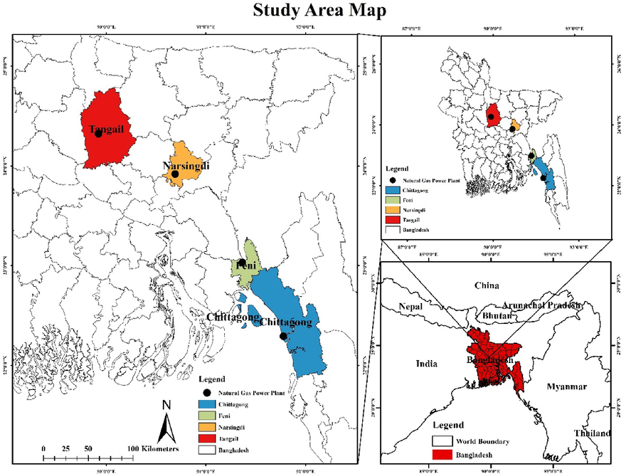

Natural gas-fired power plant locations selected for data collection.

2.2

2.2 Data collection and analysis

The study utilized two main data sets about Particulate Matter (PM) and employee health surveys. Data regarding PM_2.5 and PM₁₀ were collected month-wise from January 2015 to December 2021 using respirable dust samplers APS-113NL for PM_2.5 and APS-113BL for PM₁₀ from the ambient air near selected engine-based natural gas-fired power plants.

In developing our machine learning models for PM_2.5 and PM₁₀ concentration forecasting, we utilized this collected historical data from 2015 to 2021. To ensure model development and evaluation, we employed a training–testing split. Data from 2015 to 2019 (roughly 71.43 % of the total data) served as the training set, where the models learned the patterns within the historical information. The remaining data from 2020 to 2021 (approximately 28.57 %) functioned as the testing set, allowing an unbiased assessment of the model's generalizability and ability to predict unseen data. Finally, after training and evaluation, we leveraged the models to forecast PM_2.5 and PM₁₀ concentrations for the years 2022, 2023, and 2024. To list employee health problems, face-to-face interviews were conducted using a representative and structured questionnaire about health issues among the randomly selected 100 employees who have been working in the electricity generation plant for over two years. The analysis methods of this study are entirely based on the information extracted from four natural gas-fired power plants (72 MW Chittagong, 22 MW Feni, 22 MW Narshingdi, and 22 MW Tangail). Air Quality Index (AQI) values and PM_2.5 and PM₁₀ were collected from the previous documents of each power plant. The AQI value was processed to determine PM_2.5 and PM₁₀ values following equations (1) and (2), respectively, and the breakpoint Table (Table 1), all prescribed by environmental protection agencies (EPAs) (Cheng et al., 2007).

(1)

I_{P M 2.5} = \{(I_{high} - I_{low}) / (C_{high} - C_{low})\} \times (AQI - C_{low}) + I_{low}

(2)

I_{P M 10} = \{(I_{high} - I_{low}) / (C_{high} - C_{low})\} \times (AQI - C_{low}) + I_{low}

where I_PM2.5 = Particulate Matter 2.5 Emission (µg/m³), I_PM10 = Particulate Matter 10 Emission (µg/m³), I_high = Index breakpoint corresponding to C_high, I_low = Index breakpoint corresponding to C_low, C_high = The concentration breakpoint ≥ C, C_low = The concentration breakpoint ≤ C.

Table 1 Air quality index (AQI) and breakpoint prescribed by environmental protection agencies.

AQI	Level of health concern	PM_2.5 (µg/m³)	PM₁₀ (µg/m³)
0–50	Good	0–15.4	0–54
51–100	Moderate	15.5–40.4	55–154
101–150	Unhealthy for sensitive group	40.5–65.4	155–254
151–200	Unhealthy	65.5–150.4	255–354
201–300	Very unhealthy	150.5–250.4	355–424
301–400	Hazardous	250.5–350.4	425–504
401–500	Very hazardous	350.5–500.4	505–604

To assess health hazards due to PM, the forecasted values were compared with the EPA's breakpoint AQI value. Finally, data were recorded and analyzed using Rstudio and Microsoft Excel, and a study area map was prepared using ArcGIS software. ARIMA, ETS, and ANN models were used to analyze and forecast PM_2.5 and PM₁₀ concentrations in specific power generation plants. The analysis involved in this article has run on the R-4.0.5 workstation. This study prepared its R routines that suited the procedure adopted. Natural gas power plant data from 2015 to 2021 were analyzed using ARIMA, ETS, and ANN models for time series analysis and forecasting. While the ARIMA model is generally considered computationally efficient compared to some other time series forecasting methods, the actual computation time can vary depending on factors like data size and model complexity (p, d, q values). In larger datasets or with more complex models, computation time may increase (Hyndman and Khandakar, 2008).

2.3

2.3 Auto-Regressive Integrated Moving average (ARIMA)

Box Jenkins was used to analyze the data and forecast emissions in this study. Time series can be stationary or non-stationary, and this technique fits neatly into the category of the linear model. Box-Jenkins methods are helpful in forecasting because they include Autoregressive (AR) models, integrated (I) models, and Moving Average (MA) models. The Box-Jenkins methodology requires four steps to obtain the model: data preparation, model selection, estimation, and forecasting. A model is then employed as a prediction tool. After data collection, we first determined whether the data were part of a stationary or non-stationary time series. To identify these data, we used the augmented Dickey-Fuller (ADF) test. The differencing methodology may be used to make a time series stationary if it does not exhibit covariance stationary. The ARIMA (p, d, q) model is created by applying the ARMA (p, q) model to stationary differenced time series, where d is the order of differencing. We used the ADF test after the difference, which reveals the stationary time series. One approach for identifying trends in the data is the autocorrelation function. The autocorrelation function informs users of the correlation between points separated by different time lags. Given a sample Y0, Y1…, YT-1 of T observations, we define the sample autocorrelation function to be the sequence of values,

(3)

r τ = C τ / C 0, τ = 0, 1, . . ., T - 1

The partial autocorrelation function (PACF) in time series analysis provides the partial correlation of a time series with its own lagged values while controlling for the importance of the time series at all shorter lags. The sample partial autocorrelation Pτ at lag τ is simply the correlation between the two sets of residuals obtained from regressing the elements Yt and Yt − τ on the set of intervening values Y1, Y2, …, Yt-τ + 1. The Akaike information criterion (AIC) compares statistical model quality. The “best” model will be characterized by which doesn't fit either too well or too poorly. AIC is usually calculated with the software. The basic formula is defined as follows.

(4)

AIC = - 2 (\log - l i k e l i h o o d) + 2 K

Log-likelihood is a method for measuring the model's fit, where K is the total parameter count (model variables plus intercept). The bigger the number, the better the fit. This is usually obtained from statistical output. In statistics, the Bayesian Information Criterion (BIC) may be a criterion for model selection among a finite set of models; the model with rock-bottom BIC is preferred. It is based partly on the likelihood function, and it is closely associated with the AIC. The solution proposed by BIC and AIC is to include a penalty term for the number of parameters in the model.

2.4

2.4 Forecasting with error Trend seasonal (ETS) model

ETS point forecasting is obtained from the models by iterating the equations for

(5)

t = T + 1, \dots, T + h a n d s e t t i n g a l l ε_{t} = 0 f o r t > T

Therefore,

(6)

\bar{y} T + 1 | T = ℓ T + b T

Similarly,

(7)

yT + 2 = (ℓ T + 1 + b T + 1) (1 + ε T + 2) = [(ℓ T + b T) (1 + α ε T + 1) + b T + β (ℓ T + b T) ε T + 1] (1 + ε T + 2)

Therefore,

(8)

\bar{y} T + 2 | T = ℓ T + 2 b T

These forecasts are identical to the estimates from the model ETS as well as Holt's linear method (A, A, N). As a result, the point forecasts obtained using the technique and the two models that form its foundation are the same (assuming that the same parameter values are used). ETS point forecasts are equivalent to the forecast distributions' medians. The forecast distributions are normal for models with only additive components, so the medians and means are equal. The point forecasts and the standards of the forecast distributions will not be the same for ETS models with multiplicative errors or with multiplicative seasonality.

2.4.1

2.4.1 ETS model prediction intervals

ETS models can generate prediction intervals, but additive and multiplicative models have different prediction intervals. A prediction interval for the majority of ETS models is written as

(9)

\bar{y} T + h | T \pm c σ_{h}

Where forecasting method (A, N, A), c depends on the coverage probability, and

σ_{h}^{2}

is the forecast variance.

(10)

σ_{h}^{2} = σ^{2} [1 + α^{2} (h - 1) + γ k (2 α + γ)]

2.5

2.5 Forecasting with Artificial neural network (ANN) model

ANN is a data processing system that takes inspiration from the human brain and uses a network of many tiny processors to process data. In these networks, a programmed data structure acts like a neuron. A training algorithm is used to train a network that connects all neurons. Artificial neurons have two inputs and outputs. There are two states for every neuron: training and acting. A neuron learns the appropriate outputs for a particular input during the training phase. When information is defined for the neuron in the active state, it produces the proper output based on the training. While the hidden layer in the ANN model for PM concentration forecasting doesn't directly transmit raw data, it plays a vital role in uncovering complex patterns. It acts as a feature extractor, using non-linear activation functions to transform the lagged PM concentration values (input data) and identify underlying trends or relationships. This processed information represents a higher-level abstraction, capturing the essential features most relevant for prediction. The hidden layer then transmits this processed representation, not the raw data itself, to the output layer. Finally, the output layer leverages this learned representation to make the final prediction of future PM concentrations. In essence, the hidden layer acts as a crucial bridge, transforming the raw data into a form that the output layer uses to generate accurate forecasts.

This type of network is referred to as a multilayer feed-forward network, and it is characterized by the fact that each layer of nodes receives inputs from the layers that came before it. The inputs of the nodes in one layer come from the outputs of the nodes in the previous layer. Weighted linear combination combines each node's inputs. A nonlinear function modifies the output result.

If the inputs into hidden neuron j in Fig. 2 are combined linearly to give,

(11)

Zj = b j + \sum_{i = 1}^{4} W i, j X i

This is then adjusted using a nonlinear function, such as a sigmoid in the hidden layer so that it can act as input for the following layer. This reduces the impact of extreme input values, making the network somewhat resilient to outliers.

(12)

S (z) = \frac{1}{1 + e^{- z}}

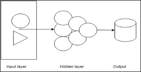
An artificial neural network (ANN) with two inputs and one hidden layer with hidden neurons.

The values of the parameters b1, b2, b3, and W1, 1,…, W4,3 are “learned” from the data. Limits are typically placed on the weight values to prevent them from becoming excessive. The value 0.1 is frequently used for the “decay parameter,” which is the parameter that controls the weight restrictions. The weights start with random values, and then those values are modified based on the data that has been observed. So, the predictions made by a neural network have a bit of a random element to them. The network is usually trained more than once using different random starting points, the results are averaged, and hidden layers and nodes are defined in advance.

2.5.1

2.5.1 Neural network autoregression (NNAR)

When using a neural network with time series data, the lag values of the time series are utilized as inputs. This study used lagged values in a linear autoregression model, called a neural network autoregression or NNAR model. This study considered feed-forward networks with one hidden layer and used the notation NNAR (p, k) to indicate there are p-lagged inputs and k nodes in the hidden layer. With seasonal data, including the most recent data from the same season as inputs is helpful, and the NNAR (p, P, k) model fits the function. If p and P are not given, a random value will be chosen for them. The default for non-seasonal time series is the optimum number of lags for a linear AR(p) model. P is set to 1 by default for seasonal time series, and p is selected from the best linear model fit to the data with seasonal adjustments. If k is left unspecified, the default value is k = (p + P + 1)/2 (rounded to the nearest integer). When it comes to making predictions, the network is used iteratively. This study simply used the available historical inputs to forecast one step. The one-step prediction was used as input to predict two steps with the previous data. This procedure continues until all the needed projections are calculated.

2.5.2

2.5.2 Prediction intervals

The foundation of neural networks is not a well-defined stochastic model; as a consequence, calculating prediction intervals for the resulting projections is difficult. However, through simulation, we have calculated prediction intervals where future sample pathways are produced using bootstrapped residuals. The neural network fitted to the PM data can be written as

(13)

y_{t} = f (y_{t} - 1) + ε_{t}

where

yt - 1 = (y t - 1, y t - 2, \dots ., y t - 10)'

is a vector containing lagged values of the series, and f is a neural network with six hidden nodes in a single layer. The error series {εt} is assumed to be homoscedastic (maybe a normal distribution). The ability to simulate future sample paths of this model repeatedly by selecting a value at random for εt, either from a normal distribution or by resampling the historical values.

So, if εT + 1 is a random draw from the distribution of errors at time T + 1, then yT + 1 = f(yT) + εT + 1 is one possible draw from the forecast distribution for yT + 1.

Setting, yT + 1 = (yT + 1, yT, …, yT − 8)′, we can then repeat the process to get yT + 2 = f(yT + 1) + εT + 2.

In this manner, this may repeatedly simulate a future sample route. This study gains knowledge of the distribution for all future values by continually forging sample routes based on the fitted neural network.

3 Results and discussion

3.1

3.1 Particulate matter (PM) concentration scenario in natural gas-fired power plant

Table 2 shows the concentration of PM_2.5 and PM₁₀ in the natural gas burning in 4 storks internal combustion engines in four power plants located in Chittagong, Feni, Narshingdi, and Tangail districts of Bangladesh, generating a yearly capacity of 1208.88 GW. PM concentrations in power plants depend on operation, fuel burning, and air filtering. Wartsila and Rolls Royce engines ensure rich burn to avoid carbon monoxide and PM emissions. This study covered four natural gas power plants in different locations to analyze PM_2.5 and PM₁₀ data from 2015 to 2021 and forecast. The concentration of PM in the atmosphere has increased day by day as a result of fuel burning and steady emissions from fossil fuel-burning power plants without filtering, construction work, or other development activities (Shin et al., 2022b). PM emissions are not directly from fuel burning and indicate ambient PM concentrations in the electricity generation area. According to EPA standards, monitored PM concentrations are unhealthy in all fossil fuel-burning power plants. PM_2.5 and PM₁₀ concentrations in selected power generation complexes have fluctuated over the past seven years, and the highest average PM_2.5 concentration was recorded in 2020, at 122.6 µg/m³. The lowest average PM_2.5 concentration was recorded in 2017, at 76.3 µg/m³. PM₁₀ concentrations generally followed a similar trend to PM_2.5 concentrations, and both PM_2.5 and PM₁₀ concentrations exceeded the EPA's standard in all years measured (Table 2).

Table 2 Particulate matter concentration status in natural gas-based power plants.

Year	*EPA's standard (µg/m³)		PM_2.5 µg/m³	PM₁₀ µg/m³
Year	PM_2.5	PM₁₀	PM_2.5 µg/m³	PM₁₀ µg/m³
2015	12–15	>150	86.8	229.3
2016			95.4	211
2017			76.3	203.3
2018			83.0	207.8
2019			126	283
2020			122.6	279
2021			88.5	225

*U.S. Environmental Protection Agency (Minh et al., 2021).

3.2

3.2 Forecasting of PM_2.5 and PM₁₀ using ARIMA, ETS, and ANN models

In time series forecasting, ensuring the data is stationary (meaning its statistical properties remain constant over time) is crucial for obtaining reliable predictions. The ADF test is a common tool used to assess stationarity. As shown in Table 3, the ADF test results for PM_2.5 and PM₁₀ both have p-values less than 0.05 (a commonly used significance level) and negative test statistics, indicating a rejection of the null hypothesis of a unit root (non-stationarity) at the chosen significance level. The p-value is less than 0.05 for both variables, a commonly used statistical significance threshold. This further supports the conclusion of stationarity. The lag order is 3 for both PM_2.5 and PM₁₀, indicating that the model used to perform the ADF test included 3 lags of the differenced data (Table 3). This shows we can reject the null hypothesis of non-stationarity, and both variables are likely stationary. With stationary data, we can proceed more confidently to our chosen forecasting model.

Table 3 Data summary of unit root tests for PM_2.5 and PM_10.

Variable	ADF test	Lag order	P-value	Alternative hypothesis
PM_2.5	−3.9076	3	0.02018	Stationary
PM₁₀	−3.9126	3	0.0212	Stationary

In this analysis of PM_2.5 and PM₁₀ concentration forecasting, ARIMA models emerged as a potentially better solution compared to ETS models based on AIC and BIC criteria. For PM_2.5, an ARIMA (1,0,0) (1,1,0) [12] model captured the influence of the previous month's value (positive coefficient) along with a seasonal effect (negative coefficient). PM₁₀ also exhibited a seasonal pattern, but its ARIMA model ARIMA (1,0,0) (2,1,0) [12] included two seasonal autoregressive terms, suggesting a more complex seasonal influence. Overall, the importance of the seasonal component was evident in both PM_2.5 and PM₁₀, while automated ARIMA models provided a better fit based on the chosen information criteria. These methods produce better prediction plots, and Fig. 4 demonstrates how accurate the predicted value was. We observed the data from 2015, 2016, 2017, and 2018 using the ARIMA model, and then we forecasted the data for 2019, 2020, and 2021. Even though we were aware of the data from 2019, 2020, and 2021, the mean absolute scaled error (MASE) value for PM_2.5 and PM₁₀ was MASE < 1, which indicates the model does not need improvement and model is exactly as good (Wang and Lu, 2018). It is possible to say, based on a rule of thumb, lower Root mean squared error (RMSE) values, demonstrate that the model can predict the data accurately. Similarly, the ETS models for PM_2.5 and PM₁₀ employed additive errors and additive trend components. ETS (M, N, M), ETS (A, N, A), and NNAR (1,1,2) [12] were used for PM_2.5 and PM₁₀ series, which gives a better prediction plot. We observed the data as before observed for the ARIMA model from 2015, 2016, 2017, and 2018 using the ETS and ANN model, and then we forecasted the data for 2019, 2020, and 2021 (Table 4). The ANN model summary suggests it's not just a single model, but an ensemble of 20 similar ANNs with 2 hidden layers, each containing 2 neurons. These networks likely have slightly different weights leading to a more robust prediction. ANN model also has the total number of trainable parameters (weights and biases) in each network within the ensemble (2 neurons in the first layer * 2 neurons in the second layer + biases = 9). The final layer of each network uses linear activation, meaning the output is a direct linear combination of the weighted inputs from the previous layer. However, the mean absolute error (MAE) of PM_2.5 from the ANN model was closer to zero than PM_2.5 from the ETS model, and PM₁₀ from the ETS model was closer to zero than PM₁₀ from the ANN model, which indicates PM_2.5 from the ANN model, and PM₁₀ from ETS model is more accurate than PM_2.5 from ETS and PM₁₀ from ANN model respectively (Eǧrioǧlu et al., 2008). According to the RMSE, MAE, MAPE (Mean absolute percentage error), and MASE values projected by the ARIMA, ETS, and ANN models, the expected value for PM concentration in natural gas-fueled power plant areas in 2022, 2023, and 2024 are accurate, and the model used for forecasting worked well. Table 4 compares the forecasts of ARIMA, ETS, and ANN models for PM_2.5 and PM₁₀ concentrations in the study area and shows the predicted concentrations for January to December in 2022, 2023, and 2024.

Table 4 Predicted values of PM concentrations (μg/m³) in natural gas-fired power plants during 2022–2024.

ARIMA Forecasting
	Year	Jan	Feb	Mar	Apr	May	Jun	July	Aug	Sep	Oct	Nov	Dec
PM_2.5	2022	203.7	155.5	129.1	42.2	27.5	19.9	14.6	73.3	65.9	76.0	178.7	214.7
	2023	223.6	140.6	122.6	53.9	30.4	25.3	14.3	80.7	45.5	65.7	151.5	181.0
	2024	212.9	148.6	126.0	47.7	28.9	22.3	14.5	76.7	56.4	67.0	166.1	199.0
PM₁₀	2022	364.5	302.5	297.0	201.7	160.0	139.5	111.6	207.3	215.2	270.6	323.6	337.5
	2023	391.1	336.7	313.5	200.4	150.3	118.1	89.5	205.4	213.6	274.9	333.9	354.3
	2024	391.3	325.2	306.4	209.6	152.7	127.2	87.5	205.8	189.0	246.7	315.7	332.7

ETS forecasting
PM_2.5	2022	191.0	149.3	110.4	40.5	30.1	20.8	14.7	41.3	41.9	45.0	98.3	157.3
	2023	191.0	149.3	110.4	40.5	30.1	20.8	14.7	41.3	42.0	45.0	98.3	157.3
	2024	149.3	110.4	40.5	30.1	20.8	14.7	41.3	40.0	45.0	98.3	157.3	199.0
PM₁₀	2022	363.6	314.9	278.9	147.9	110.5	64.4	41.5	74.3	118.4	170.5	252.6	298.6
	2023	363.6	314.9	278.9	147.9	110.5	64.4	41.5	74.3	118.4	170.5	252.6	298.6
	2024	363.6	314.9	278.9	147.9	110.5	64.4	41.5	74.3	118.4	170.5	252.6	298.6

ANN forecasting
PM_2.5	2022	179.0	174.3	155.0	100.4	87.4	75.7	62.0	62.8	49.5	42.5	70.5	121.7
	2023	170.9	183.0	194.6	153.7	102.4	84.1	68.5	60.9	52.6	45.0	47.5	64.4
	2024	122.5	175.3	185.4	195.0	156.8	101.4	85.7	69.3	58.9	50.0	44.7	45.6
PM₁₀	2022	367.8	366.8	365.0	245.0	233.3	219.6	150.8	126.0	111.7	119.8	219.9	237.9
	2023	269.1	345.1	367.6	265.0	232.0	137.2	121.0	110.8	105.7	106.1	124.4	123.9
	2024	170.9	238.1	269.1	290.3	234.5	220.2	136.5	111.7	104.9	103.6	106.5	107.0

In Fig. 3, the x-axis of the graphs is time, ranging from 2015 to 2025. The y-axis is PM_2.5 or PM₁₀ concentration, measured in micrograms per cubic meter (μg/m³). The forecasts from the four models are shown as lines on the graphs. The solid line is the forecast, and the shaded area around the line represents the uncertainty of the forecast. The wider the shaded area, the less certain the forecast is. All three models predict that PM_2.5 and PM₁₀ concentrations will be highest in the winter months (December to February) and lowest in the summer months (June to August) (Fig. 3). The ARIMA model generally predicts the highest concentrations of PM_2.5 and PM₁₀, followed by the ETS model and then the ANN model. The ETS model tends to predict the most stable concentrations of PM_2.5 and PM₁₀ throughout the year, with less variation between months. The ANN model tends to predict the most volatile concentrations of PM_2.5 and PM₁₀, with the most variation between months.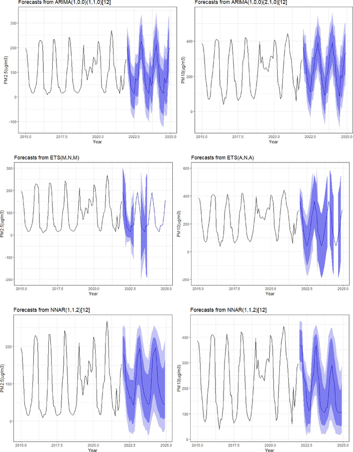

Predicted vs. observed PM2.5 and PM10 values using ARIMA, ETS, and ANN models.

3.3

3.3 Accuracy between the observed value and the predicted value of PM_2.5 and PM₁₀

Data on PM concentrations used to train ARIMA, ETS, and ANN models for modeling time series. The plots demonstrate that an ARIMA, ETS, or ANN model can be used to explain the observed time series. Fig. 4 displays, however, the degree of accuracy by the predicted value. To calculate the accuracy rate, we observed the data for 2015 to 2019 and forecasted data for 2020 and 2021. Though we knew the data for 2020 and 2021 (Fig. 4), the accuracy rate for PM_2.5 and PM₁₀ was good enough for the black line (Fig. 4), indicating observation, and the blue line for prediction.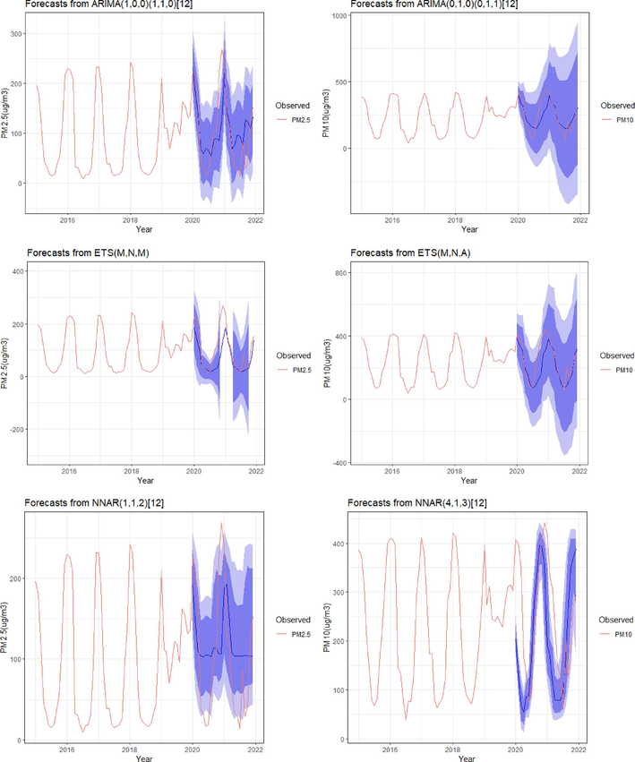

Observed value vs. predicted value plot (accuracy of prediction).

Table 5 compares the performance of three different models named ARIMA, ETS, and ANN for predicting the concentration of two pollutants, PM_2.5 and PM₁₀. It uses four different error measures RMSE, MAE, MAPE, and MASE, and a lower value indicates better performance. Overall, ANN and ARIMA seem to have comparable performance for PM_2.5 prediction based on RMSE and MAE. Both have very similar values. MAPE is slightly higher for ANN, while MASE is slightly lower. For PM₁₀ prediction, ANN might perform slightly worse than ARIMA based on RMSE and MAE. The difference is small though. MAPE is again slightly higher for ANN, while MASE is comparable. ETS seems to perform worse than both ARIMA and ANN for both pollutants based on all error measures. It has higher values for RMSE, MAE, MAPE, and MASE for both PM_2.5 and PM₁₀. MAPE greater than 10 % but less than 25 % was found in ARIMA, ETS, and ANN models for PM₁₀ and indicates low but acceptable accuracy, and MAPE for PM_2.5 in all models is above 25 %, suggesting a relatively poor fit for predicting PM_2.5 concentrations. MASE is below 1 and indicates the model used in forecasting data shows forecasting performance was good.

Table 5 Error measure for the predicted value of ARIMA, ETS, and ANN models.

Models	Pollutants	RMSE	MAE	MAPE	MASE	R²
ARIMA	PM_2.5	36.69	0.247	39.8	0.57	0.56
ARIMA	PM₁₀	48.49	0.363	20.26	0.59	0.062

ETS	PM_2.5	49.07	0.306	38.25	0.70	0.64
ETS	PM₁₀	44.60	0.355	19.26	0.57	−0.10

ANN	PM_2.5	36.63	0.283	45.94	0.65	0.89
ANN	PM₁₀	46.59	0.388	22.47	0.63	−0.01

N. B.: ARIMA = Auto-Regressive Integrated Moving Average, ETS = Error Trend Seasonal, ANN = Artificial Neural Network, RMSE = Root mean squared error, MAE = mean absolute error, MAPE = Mean absolute percentage error, MASE = mean absolute scaled error, R² = Coefficient of Determination.

In addition, R² yielded promising results for PM_2.5 prediction. The ARIMA model captured a moderate amount of variance (R² = 0.56), which means it explains a decent portion of the fluctuations in PM_2.5 levels. The ETS model performed even better (R² = 0.64), effectively capturing trends and seasonal patterns. The ANN model emerged as the leader (R² = 0.89), explaining a very high proportion of the variance in PM_2.5 data. In statistical terms, an R2 of 1 indicates a perfect fit, while 0 signifies the model doesn't explain any variance. Therefore, the ANN model seems adept at capturing complex relationships in PM_2.5 data that other models might miss. However, PM₁₀ prediction remains a challenge. Both ARIMA and ETS models underperformed (R² < 0.06), suggesting they may not be suitable for capturing the patterns in PM₁₀ concentrations. The ANN model also exhibited a negative R², indicating its forecasts were on average worse than simply using the historical average PM₁₀ value. Further investigation is necessary to identify a more effective model for PM₁₀ prediction.

3.4

3.4 Health impact assessment of particulate matter from natural gas-fired power plant

Electricity generation and fuel consumption are connected with air emissions from natural gas-fired power plants. Electricity utilities are regulated at the national level under DoE rules and regulations. Emissions from power plants pose a potentially considerable risk to human health and the environment. These pollution sources are of particular concern in Bangladesh, where the burning of natural gas generates a large share of electricity. There are a variety of effects on human health depending on the content of air pollutants, the quantity, and duration of exposure, and the fact that people are often exposed to combinations of pollutants rather than single ones. Health consequences on people might include anything from cancer to nausea and respiratory problems. People working in a power plant exposed to emissions face health issues like breathing or skin irritation at a higher than the community people (Kampa and Castanas, 2008). Health effects can be distinguished into acute and chronic, not including cancer and cancerous. Epidemiological and animal model studies show that the cardiovascular and respiratory systems are predominantly impacted by the exposure (Pinkerton et al., 2019). Fig. 5 shows the yearly average air pollution level, including forecasted pollution mean level compared with AQI value and associated health risks in NG-fired power plants.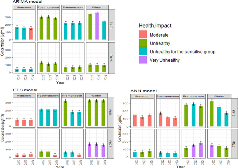

The forecasted health impact of PM2.5 and PM10 concentration in natural gas power plants.

However, this research separated the year into four distinct seasons: winter (March-May), pre-monsoon (June-August), post-monsoon (September-November), and monsoon (December- February). Applying the ARIMA model to the data on PM_2.5, it was predicted that during the monsoon season, natural gas-fired power plants will be unhealthy for sensitive groups in 2022, 2023, and 2024. The health hazard from PM₁₀ will be moderate in the 2024 monsoon season. ETS forecasting for 2022, 2023, and 2024 indicates that the health risk from PM_2.5 will be moderate in the monsoon season, and in the winter, the health risk will be very unhealthy in the power-generating site. According to the ANN forecasting model, due to PM_2.5, health hazards will be very unhealthy for the sensitive group in the pre-monsoon season of 2023 and 2024 and in the winter season of 2022 (Fig. 5). Digging deep into the health of natural gas-fired power plant workers, interviewed 100 employees. The results were alarming, 15 % reported grappling with health issues directly linked to the power plant's air quality. This translated to 2 % struggling with respiratory problems and even higher 13 % bore the visible marks of poor air quality on their skin, with rashes and irritation a constant reminder of their occupational hazard. These statistics underscore the urgent need for stricter air quality regulations and better protective measures for power plant workers. However, implementing regular health checks, air filtration systems, and renewable energy consumption can provide a multitude of benefits for the environment. These practices promote healthier living, reduce environmental pollution, and contribute to a more sustainable future (Martínez-Mendoza et al., 2022).

4 Conclusions

This study investigated PM_2.5 and PM₁₀ concentrations near natural gas-fired power plants using time series analysis and forecasting models ARIMA, ETS, and ANN to assess potential health risks associated with PM exposure and predict future air quality. Our findings revealed a link between PM concentrations and potential health problems like respiratory issues, heart disease, and premature death, aligning with established scientific evidence from the EPA. These results highlight the need for stricter PM control strategies to safeguard human health and environmental quality around these types of power plants.

5 Availability of data and material

The datasets used or analyzed during the current study are available from the first author upon reasonable request.

Funding

This research was funded by the research grants of Research Cell, Noakhali Science and Technology University (No. NSTU/RC/MS/21/131).

CRediT authorship contribution statement

Mustafizur Rahman: Writing – review & editing, Writing – original draft, Software, Methodology, Formal analysis, Data curation, Conceptualization. Kamrul Hasan: Visualization, Software, Formal analysis. Md. Abu Bakar Siddique: Writing – review & editing, Investigation. Balram Ambade: Writing – review & editing, Investigation. Md. Alamgir Hussain: Writing – review & editing. Mohammed Abdus Salam: Writing – review & editing, Supervision, Investigation, Funding acquisition. Salman Tariq: Writing – review & editing. Muhammad Ibrahim: Writing – review & editing.

Declaration of competing interest

The authors declare that they have no known competing financial interests or personal relationships that could have appeared to influence the work reported in this paper.

References

Abdul Jameel A.G., Elbaz A.M., Emwas A.H., Roberts W.L., Sarathy S.M., . Calculation of average molecular parameters, functional groups, and a surrogate molecule for heavy fuel oils using 1H and 13C nuclear magnetic resonance spectroscopy. Energy Fuels. 2016;30:3894-3905.
[CrossRef] [Google Scholar]
Al-Amin M., Sahabuddin M., . High penetration of electric autorickshaw on national power system and barriers against the adoption of solar energy: a case study in Bangladesh. Clean Eng. Technol.. 2023;14
[CrossRef] [Google Scholar]
Anam K., Husnain-Al-Bustam, . Power crisis & its solution through renewable energy in bangladesh. journal of selected areas in renewable and sustainable. Energy 2011:13-18.
[Google Scholar]
Bai L., Wang J., Ma X., Lu H., . Air pollution forecasts: an overview. Int. J. Environ. Res. Public Health 2018
[CrossRef] [Google Scholar]
BBS, SID, MoF, 2017. Bangladesh Statistics 2016. Bangladesh Bureau of Statistics Statistics and Informatics Division Ministry of Planning 73.
Begum, B.A., Saroar, G., Nasiruddin, M., Randal, S., Sivertsen, B., Hopke, P.K., 2014a. Particulate Matter and Black Carbon Monitoring at Urban Environment in Bangladesh. NUCLEAR SCIENCE AND APPLICATIONS 23.
Begum B.A., Saroar G., Nasiruddin M., Randal S., Sivertsen B., Hopke P.K., . Particulate matter and black carbon monitoring at urban environment in Bangladesh. Nucl. Sci. Appl.. 2014;23:1-8.
[Google Scholar]
Cellura M., Cusenza M.A., Longo S., . Energy-related GHG emissions balances: IPCC versus LCA. Sci. Total Environ.. 2018;628–629:1328-1339.
[CrossRef] [Google Scholar]
Cheng W.L., Chen Y.S., Zhang J., Lyons T.J., Pai J.L., Chang S.H., . Comparison of the revised air quality index with the PSI and AQI indices. Sci. Total Environ.. 2007;382:191-198.
[CrossRef] [Google Scholar]
Chowdhury A.I., Uddin M.J., Baul T.K., Akhter J., Nandi R., Karmakar S., Nath T.K., . Quantifying the potential contribution of urban trees to particulate matters removal: a study in Chattogram city, Bangladesh. J. Clean. Prod.. 2022;380:135015
[CrossRef] [Google Scholar]
Eǧrioǧlu E., Aladaǧ Ç.H., Günay S., . A new model selection strategy in artificial neural networks. Appl. Math. Comput.. 2008;195:591-597.
[CrossRef] [Google Scholar]
Ghenai, C., Bettayeb, M., 2021. Data analysis of the electricity generation mix for clean energy transition during COVID-19 lockdowns. Energy Sources, Part A: Recovery, Utilization and Environmental Effects. 10.1080/15567036.2021.1884772.
Ghosh S., . Electricity consumption and economic growth in India. Energy Policy. 2002;30:125-129.
[Google Scholar]
Gu, Y., Yan, F., Xu, J., Duan, Y., Fu, Q., Qu, Y., Liao, H., 2021. Mitigated PM2.5 Changes by the Regional Transport During the COVID‐19 Lockdown in Shanghai, China. Geophys. Res. Lett. 48. 10.1029/2021GL092395.
Holechek J.L., Geli H.M.E., Sawalhah M.N., Valdez R., . A global assessment: can renewable energy replace fossil fuels by 2050? Sustainability (Switzerland). 2022;14
[CrossRef] [Google Scholar]
Ibe F.C., Opara A.I., Duru C.E., Obinna I.B., Enedoh M.C., . Statistical analysis of atmospheric pollutant concentrations in parts of Imo State, Southeastern Nigeria. Sci. Afr.. 2020;7
[CrossRef] [Google Scholar]
Islam A., Ahmed M.T., Mondal M.A.H., Awual M.R., Monir M.U., Islam K., . A snapshot of coal-fired power generation in Bangladesh: a demand–supply outlook. Nat. Resour. Forum.. 2021;45:157-182.
[CrossRef] [Google Scholar]
Islam S., Khan M.Z.R., . A review of energy sector of bangladesh. Energy Proc.. 2017;110:611-618.
[CrossRef] [Google Scholar]
Kampa M., Castanas E., . Human health effects of air pollution. Environ. Pollut. 2008
[CrossRef] [Google Scholar]
Kim D., Han H., Wang W., Kang Y., Lee H., Kim H.S., . Application of deep learning models and network method for comprehensive air-quality index prediction. Appl. Sci. (Switzerland). 2022;12
[CrossRef] [Google Scholar]
Markandya, A., Wilkinson, P., 2007. Energy and Health 2 Electricity generation and health. www.thelancet.com 370. 10.1016/S0140.
Martínez-Mendoza, E., Fernández-Echeverría, E., García-Santamaría, L.E., Ruvalcaba-Sánchez, L. and Fernández Lambert, G., 2022. Wind Farms Waste: Non-Calculated Environmental Impact?. Available at SSRN 4043654.
Minh V.T.T., Tin T.T., Hien T.T., . PM2.5 forecast system by using machine learning and WRF Model, A Case Study: Ho Chi Minh City, Vietnam. Aerosol. Air Qual. Res.. 2021;21:210108
[CrossRef] [Google Scholar]
Pinkerton K.E., Chen C.Y., Mack S.M., Upadhyay P., Wu C.W., Yuan W., . Cardiopulmonary health effects of airborne particulate matter: correlating animal toxicology to human epidemiology. Toxicol. Pathol.. 2019;47:954-961.
[CrossRef] [Google Scholar]
PSMP 2016, Power Division, Ministry of Power, Energy and Mineral Resources. Government of the People's Republic of Bangladesh.
Qu C.S., Ma Z.W., Yang J., Liu Y., Bi J., Huang L., . Human exposure pathways of heavy metals in a lead-zinc mining area, jiangsu province. China. Plos One. 2012;7
[CrossRef] [Google Scholar]
Radojević D., Pocajt V., Popović I., Perić-Grujić A., Ristić M., . Forecasting of greenhouse gas emissions in serbia using artificial neural networks. Energy Sources, Part a: Recovery, Utilization and Environmental Effects. 2013;35:733-740.
[CrossRef] [Google Scholar]
Rahman M., Rashid F., Roy S.K., Habib M.A., . Application of extreme learning machine (ELM) forecasting model on CO2 emission dataset of a natural gas-fired power plant in Dhaka. Bangladesh. Data Brief. 2024;54:110491
[CrossRef] [Google Scholar]
Rashid F., Joardder M.U.H., . Future options of electricity generation for sustainable development: trends and prospects. Eng. Rep. 2022
[CrossRef] [Google Scholar]
Shahriar S.A., Kayes I., Hasan K., Salam M.A., Chowdhury S., . Applicability of machine learning in modeling of atmospheric particle pollution in Bangladesh. Air Qual. Atmos. Health. 2020;13:1247-1256.
[CrossRef] [Google Scholar]
Shin, D., Kim, Y., Hong, K.J., Lee, G., Park, I., Kim, H.J., Kim, Y.J., Han, B., Hwang, J., 2022a. Measurement and Analysis of PM10 and PM2.5 from Chimneys of Coal-fired Power Plants Using a Light Scattering Method. Aerosol Air Qual Res 22. 10.4209/AAQR.210378.
Shin, D., Kim, Y., Hong, K.J., Lee, G., Park, I., Kim, H.J., Kim, Y.J., Han, B., Hwang, J., 2022b. Measurement and Analysis of PM10 and PM2.5 from Chimneys of Coal-fired Power Plants Using a Light Scattering Method. Aerosol Air Qual Res 22. 10.4209/AAQR.210378.
Sokulski C.C., Barros M.V., Salvador R., Broday E.E., de Francisco A.C., . Trends in renewable electricity generation in the g20 countries: an analysis of the 1990–2020 period. Sustainability (switzerland). 2022;14
[CrossRef] [Google Scholar]
Thabani N., Wellington G., Bonga, . Prediction of Emissions in India using ARIMA Models. DRJ J. Econ. Finance. 2019
[Google Scholar]
Vultaggio M., Varrica D., Alaimo M.G., . Impact on air quality of the COVID-19 lockdown in the urban area of palermo (Italy) Int. J. Environ. Res. Public Health. 2020;17:7375.
[CrossRef] [Google Scholar]
Wang W., Lu Y., . Analysis of the Mean Absolute Error (MAE) and the Root Mean Square Error (RMSE) in Assessing Rounding Model. Institute of Physics Publishing; 2018.
[CrossRef]
Woodward A., Smith K.R., Campbell-Lendrum D., Chadee D.D., Honda Y., Liu Q., Olwoch J., Revich B., Sauerborn R., Chafe Z., Confalonieri U., Haines A., . Climate change and health: On the latest IPCC report. The Lancet 2014
[CrossRef] [Google Scholar]

Show Sections

[1] Abdul Jameel A.G., Elbaz A.M., Emwas A.H., Roberts W.L., Sarathy S.M., . Calculation of average molecular parameters, functional groups, and a surrogate molecule for heavy fuel oils using 1H and 13C nuclear magnetic resonance spectroscopy. Energy Fuels. 2016;30:3894-3905.
[CrossRef] [Google Scholar]

[2] Al-Amin M., Sahabuddin M., . High penetration of electric autorickshaw on national power system and barriers against the adoption of solar energy: a case study in Bangladesh. Clean Eng. Technol.. 2023;14
[CrossRef] [Google Scholar]

[3] Anam K., Husnain-Al-Bustam, . Power crisis & its solution through renewable energy in bangladesh. journal of selected areas in renewable and sustainable. Energy 2011:13-18.
[Google Scholar]

[4] Bai L., Wang J., Ma X., Lu H., . Air pollution forecasts: an overview. Int. J. Environ. Res. Public Health 2018
[CrossRef] [Google Scholar]

[5] BBS, SID, MoF, 2017. Bangladesh Statistics 2016. Bangladesh Bureau of Statistics Statistics and Informatics Division Ministry of Planning 73.

[6] Begum, B.A., Saroar, G., Nasiruddin, M., Randal, S., Sivertsen, B., Hopke, P.K., 2014a. Particulate Matter and Black Carbon Monitoring at Urban Environment in Bangladesh. NUCLEAR SCIENCE AND APPLICATIONS 23.

[7] Begum B.A., Saroar G., Nasiruddin M., Randal S., Sivertsen B., Hopke P.K., . Particulate matter and black carbon monitoring at urban environment in Bangladesh. Nucl. Sci. Appl.. 2014;23:1-8.
[Google Scholar]

[8] Cellura M., Cusenza M.A., Longo S., . Energy-related GHG emissions balances: IPCC versus LCA. Sci. Total Environ.. 2018;628–629:1328-1339.
[CrossRef] [Google Scholar]

[9] Cheng W.L., Chen Y.S., Zhang J., Lyons T.J., Pai J.L., Chang S.H., . Comparison of the revised air quality index with the PSI and AQI indices. Sci. Total Environ.. 2007;382:191-198.
[CrossRef] [Google Scholar]

[10] Chowdhury A.I., Uddin M.J., Baul T.K., Akhter J., Nandi R., Karmakar S., Nath T.K., . Quantifying the potential contribution of urban trees to particulate matters removal: a study in Chattogram city, Bangladesh. J. Clean. Prod.. 2022;380:135015
[CrossRef] [Google Scholar]

[11] Eǧrioǧlu E., Aladaǧ Ç.H., Günay S., . A new model selection strategy in artificial neural networks. Appl. Math. Comput.. 2008;195:591-597.
[CrossRef] [Google Scholar]

[12] Ghenai, C., Bettayeb, M., 2021. Data analysis of the electricity generation mix for clean energy transition during COVID-19 lockdowns. Energy Sources, Part A: Recovery, Utilization and Environmental Effects. 10.1080/15567036.2021.1884772.

[13] Ghosh S., . Electricity consumption and economic growth in India. Energy Policy. 2002;30:125-129.
[Google Scholar]

[14] Gu, Y., Yan, F., Xu, J., Duan, Y., Fu, Q., Qu, Y., Liao, H., 2021. Mitigated PM2.5 Changes by the Regional Transport During the COVID‐19 Lockdown in Shanghai, China. Geophys. Res. Lett. 48. 10.1029/2021GL092395.

[15] Holechek J.L., Geli H.M.E., Sawalhah M.N., Valdez R., . A global assessment: can renewable energy replace fossil fuels by 2050? Sustainability (Switzerland). 2022;14
[CrossRef] [Google Scholar]

[16] Ibe F.C., Opara A.I., Duru C.E., Obinna I.B., Enedoh M.C., . Statistical analysis of atmospheric pollutant concentrations in parts of Imo State, Southeastern Nigeria. Sci. Afr.. 2020;7
[CrossRef] [Google Scholar]

[17] Islam A., Ahmed M.T., Mondal M.A.H., Awual M.R., Monir M.U., Islam K., . A snapshot of coal-fired power generation in Bangladesh: a demand–supply outlook. Nat. Resour. Forum.. 2021;45:157-182.
[CrossRef] [Google Scholar]

[18] Islam S., Khan M.Z.R., . A review of energy sector of bangladesh. Energy Proc.. 2017;110:611-618.
[CrossRef] [Google Scholar]

[19] Kampa M., Castanas E., . Human health effects of air pollution. Environ. Pollut. 2008
[CrossRef] [Google Scholar]

[20] Kim D., Han H., Wang W., Kang Y., Lee H., Kim H.S., . Application of deep learning models and network method for comprehensive air-quality index prediction. Appl. Sci. (Switzerland). 2022;12
[CrossRef] [Google Scholar]

[21] Markandya, A., Wilkinson, P., 2007. Energy and Health 2 Electricity generation and health. www.thelancet.com 370. 10.1016/S0140.

[22] Martínez-Mendoza, E., Fernández-Echeverría, E., García-Santamaría, L.E., Ruvalcaba-Sánchez, L. and Fernández Lambert, G., 2022. Wind Farms Waste: Non-Calculated Environmental Impact?. Available at SSRN 4043654.

[23] Minh V.T.T., Tin T.T., Hien T.T., . PM2.5 forecast system by using machine learning and WRF Model, A Case Study: Ho Chi Minh City, Vietnam. Aerosol. Air Qual. Res.. 2021;21:210108
[CrossRef] [Google Scholar]

[24] Pinkerton K.E., Chen C.Y., Mack S.M., Upadhyay P., Wu C.W., Yuan W., . Cardiopulmonary health effects of airborne particulate matter: correlating animal toxicology to human epidemiology. Toxicol. Pathol.. 2019;47:954-961.
[CrossRef] [Google Scholar]

[25] PSMP 2016, Power Division, Ministry of Power, Energy and Mineral Resources. Government of the People's Republic of Bangladesh.

[26] Qu C.S., Ma Z.W., Yang J., Liu Y., Bi J., Huang L., . Human exposure pathways of heavy metals in a lead-zinc mining area, jiangsu province. China. Plos One. 2012;7
[CrossRef] [Google Scholar]

[27] Radojević D., Pocajt V., Popović I., Perić-Grujić A., Ristić M., . Forecasting of greenhouse gas emissions in serbia using artificial neural networks. Energy Sources, Part a: Recovery, Utilization and Environmental Effects. 2013;35:733-740.
[CrossRef] [Google Scholar]

[28] Rahman M., Rashid F., Roy S.K., Habib M.A., . Application of extreme learning machine (ELM) forecasting model on CO2 emission dataset of a natural gas-fired power plant in Dhaka. Bangladesh. Data Brief. 2024;54:110491
[CrossRef] [Google Scholar]

[29] Rashid F., Joardder M.U.H., . Future options of electricity generation for sustainable development: trends and prospects. Eng. Rep. 2022
[CrossRef] [Google Scholar]

[30] Shahriar S.A., Kayes I., Hasan K., Salam M.A., Chowdhury S., . Applicability of machine learning in modeling of atmospheric particle pollution in Bangladesh. Air Qual. Atmos. Health. 2020;13:1247-1256.
[CrossRef] [Google Scholar]

[31] Shin, D., Kim, Y., Hong, K.J., Lee, G., Park, I., Kim, H.J., Kim, Y.J., Han, B., Hwang, J., 2022a. Measurement and Analysis of PM10 and PM2.5 from Chimneys of Coal-fired Power Plants Using a Light Scattering Method. Aerosol Air Qual Res 22. 10.4209/AAQR.210378.

[32] Shin, D., Kim, Y., Hong, K.J., Lee, G., Park, I., Kim, H.J., Kim, Y.J., Han, B., Hwang, J., 2022b. Measurement and Analysis of PM10 and PM2.5 from Chimneys of Coal-fired Power Plants Using a Light Scattering Method. Aerosol Air Qual Res 22. 10.4209/AAQR.210378.

[33] Sokulski C.C., Barros M.V., Salvador R., Broday E.E., de Francisco A.C., . Trends in renewable electricity generation in the g20 countries: an analysis of the 1990–2020 period. Sustainability (switzerland). 2022;14
[CrossRef] [Google Scholar]

[34] Thabani N., Wellington G., Bonga, . Prediction of Emissions in India using ARIMA Models. DRJ J. Econ. Finance. 2019
[Google Scholar]

[35] Vultaggio M., Varrica D., Alaimo M.G., . Impact on air quality of the COVID-19 lockdown in the urban area of palermo (Italy) Int. J. Environ. Res. Public Health. 2020;17:7375.
[CrossRef] [Google Scholar]

[36] Wang W., Lu Y., . Analysis of the Mean Absolute Error (MAE) and the Root Mean Square Error (RMSE) in Assessing Rounding Model. Institute of Physics Publishing; 2018.
[CrossRef]

[37] Woodward A., Smith K.R., Campbell-Lendrum D., Chadee D.D., Honda Y., Liu Q., Olwoch J., Revich B., Sauerborn R., Chafe Z., Confalonieri U., Haines A., . Climate change and health: On the latest IPCC report. The Lancet 2014
[CrossRef] [Google Scholar]

Particulate matter concentrations around natural gas-fired power plants and their associated health impact assessment