Optimal control of a stochastic production-inventory model with deteriorating items

Ahmad M. Alshamrani

doi:10.1016/j.jksus.2012.01.004

View/Download PDF

Buy Reprints

PDF

Translate this page into:

Original Article

25 (

); 7-13

doi:

10.1016/j.jksus.2012.01.004

Optimal control of a stochastic production-inventory model with deteriorating items

Ahmad M. Alshamrani^*

Department of Statistics and Operations Research, College of Science, King Saud University, P.O. Box 2455, Riyadh 11451, Saudi Arabia

*Tel.: +966 14676279; fax: +966 14676274 ahmadm@ksu.edu.sa (Ahmad M. Alshamrani)

Received: 2011-10-22, Accepted: 2012-1-24, Published: 2012-01-01

Disclaimer:
This article was originally published by Elsevier and was migrated to Scientific Scholar after the change of Publisher.

Available online 1 February 2012

Peer review under responsibility of King Saud University.

Abstract

This paper considers a stochastic optimal control of an inventory model with a deterministic rate of deteriorating items. The dynamics of the inventory model includes a perturbation by a Wiener process. The paper uses Hamilton–Jacobi–Bellman principle to find a nonlinear partial differential equation that the value function must satisfy. The partial differential equation is solved by assuming a particular form for the solution and finding three functions Q(t), M(t), and R(t) of time by substituting the assumed solution form back in the partial differential equation. The paper then proceeds to find the optimal expected production rate and the optimal expected inventory level. The paper discusses some special cases for specific parameter values and provides some numerical examples.

Keywords

Expected inventory level

Current value function

Expected total cost

Deteriorating items

Show Related Articles from PubMed

1 Introduction

Including stochastic elements in planning problems is more realistic than simple deterministic analysis. Therefore, the framework used in this paper, the stochastic optimal control, are well suited for addressing many general problems including inventory control problems. The literature on the inventory models with deteriorating items has been around for decades, leading to survey papers such as Goyal and Giri (2001). There have also been papers that combine the idea of deteriorating inventory items with optimal control such as Benkherouf and Aggoun (2002). In this paper, we study a stochastic optimal control of a production-inventory model with deteriorating items in the presence of random disturbances.

Stochastic control problems seem to be a simple idea of nudging a stochastic process in one direction or another as it flows through time. However, the developments in this field have been multifaceted and it is therefore useful to have a framework for the discussion. The framework to be used here is outlined in Kendrick (2005) and Kendrick and Amman (2006), which provides a classification system for the stochastic control models that are used in economics.

There are two principal attributes used in Sethi and Thompson (2000) to classify economics stochastic control models, which are the stochastic elements and the solution method. Models with no stochastic elements are called deterministic. Among the models with stochastic elements, the least complexes are those with a single uncertain vector, namely additive noise terms. More complicated models which have uncertain parameters can be found in Kendrick (2005), such as measurement errors, uncertain initial state vectors, and time-varying parameters.

In a deterministic inventory system, it is assumed that the values of the state variable can be measured. In many cases, the assumption that the value of a state variable can be directly measured and exactly determined may be not realistic. In fact, the stochastic description of the production planning model is more realistic than deterministic description (Sethi and Thompson, 2000).

In the stochastic optimal control theory, the state of the system is represented by a controlled stochastic process. Therefore, the involvement of time in the state of the system will be described as a stochastic differential equation. In this paper we will only consider a stochastic differential equation of a type known as Itô equation. This equation arises when the state equation is perturbed by a Markov diffusion process (Davis, 1994; El-Gohary, 2005; Yin et al., 2003 ).

A related model was discussed by Presman and Sethi (2006) where the demand process is made up of a continuous part and a compound Poisson process. They have shown that the (s, S) policy is optimal by using an appropriate potential function. This function is then shown to satisfy the dynamic programing associated with the problem. Also, Benkherouf and Johnson (2009) examined the stochastic single item continuous review inventory model with a fixed ordering cost and where the demand is driven by a special type of a piecewise Markov deterministic process.

In this paper, we will be concerned with a stochastic production-inventory model with deteriorating items. We initially mention a related stochastic model which has been treated in Sethi and Thompson (2000), which can be derived as a special case of the model we study in this paper. Such a model can be applied to a system subjected to random disturbances. For instance, sales may follow a stochastic process which affects the deterministic inventory model.

The problem of production-inventory planning is one of the Operations Research and Management Science problems that have received a considerable amount of attention. Applications on the optimal production-inventory planning are also widely reported in the literature, see for example (Kenné and Gharbi, 2004; Parlar, 1985; Perkins and Kumar, 1994; Yang et al., 1999 ).

Shen (1994) argues that uncertainty in a stochastic control model could be classified into three categories: the first is system uncertainty, the second is parameter uncertainty, and the third is measurement uncertainty. In this paper, we assume a system uncertainty and model this by adding a random error term to the system state equation. The optimal production rate and optimal inventory level will be discussed. The problem is to find the expected optimal production rate over the planning horizon. In Section 3, the general solution of the optimal control problem will be derived. In Section 4, illustration examples and numerical examples are presented for different cases of demand rates.

2 The stochastic production-inventory model

We consider a controlled dynamic system that is affected by random noises. We aim to find strategies that minimize the expected cost over a finite time horizon while satisfying a number of constraints.

In this section, we will construct and then solve the stochastic optimal control of a production-inventory model with deterministic deteriorating items. We will introduce the possibility of controlling a system governed by Itô stochastic differential equation. We then obtain optimal states estimation for a linear system with noise.

2.1

2.1 Stochastic optimal control

This subsection is devoted to the model assumptions. We introduce the mathematical description of the problem of stochastic production-inventory system with deteriorating items. Consider a factory producing a homogeneous products that it stores in an inventory warehouse. The problem statement and notation will be introduced. Let us define the following quantities:

X(t)	stochastic inventory level at time t (state variable)
U(t)	stochastic production rate at time t (control variable)
S(t)	demand rate at time t (exogenous function)
T	length of the planning period
x₁	factory-inventory goal level
u₁	factory-production goal rate
x₀	initial inventory level
h	inventory holding cost coefficient
c	production cost coefficient
B	salvage value per unit of the inventory at time T
z(t)	standard Wiener process
σ	diffusion coefficient
θ	the deterioration coefficient

The stochastic state equation of this model can be expressed as the Itô stochastic differential equation

(2.1)

dX (t) = [U (t) - S (t) - θ X (t)] dt + σ dz (t), X (0) = x_{0},

where x₀ is the initial inventory level. The Wiener process z_t can be expressed as w(t)dt where w(t) is a white noise process (Kendrick and Amman, 2006). Now the problem is to find the optimal production rate U_t that minimizes the expected total cost. In other words, we need to find the control function U_t that maximizes the expected revenue

(2.2)

\max_{U (t)} E \{\int_{0}^{T} [- c {(U (t) - u_{1})}^{2} - h {(X (t) - x_{1})}^{2}] dt + {BX}_{T}\},

It can be shown that the integrand of the objective function (2.2) is a negative definite form. The parameters x₁ and u₁ that represent the factory-inventory goal level and factory-production goal rate can be selected by the firm.

In this study, we do not restrict our attention to non-negative production rate as required in the deterministic system. Therefore, we do not restrict production rate to be non-negative. The solution of this problem will be carried out via the Hamilton–Jacobi–Bellman principle for stochastic differential equation of the Itô type.

2.2

2.2 General solution of the problem

In this subsection, we obtain the optimal production rate that minimizes the holding and production costs. Hamilton–Jacobi equation for a certain value function which represents the minimum value of the expected total cost of the system will be derived. The model of this paper is a nice extension for the stochastic model presented in Sethi and Thompson (2000).

Let us assume that V(x, t) denotes the minimum value of the expected total cost from time t to the end of the planning horizon T with X_t = x and using the optimal policy from t to T. This function is referred to as the current value function and it should satisfy the Hamilton–Jacobi–Bellman equation in the form (Sethi and Thompson, 2000; Davis, 1994):

(2.3)

\max_{u} \{\frac{\partial V}{\partial t} + (u - S (t) - θ x) \frac{\partial V}{\partial x} + \frac{1}{2} σ^{2} \frac{\partial^{2} V}{\partial x^{2}} - c {(u - u_{1})}^{2} - h {(x - x_{1})}^{2}\} = 0,

with boundary condition

(2.4)

V (x, T) = Bx,

Differentiating the expression in Eq. (2.3) partially with respect to u and setting it equals to zero, we obtain

(2.5)

\frac{\partial V}{\partial x} - 2 c (u - u_{1}) = 0,

Therefore the optimal production rate that minimizes the total cost can be expressed as a function of the current value function in the form:

(2.6)

u (x, t) = u_{1} + \frac{1}{2 c} \frac{\partial V}{\partial x},

Substituting from (2.6) into (2.3) yields the following equation:

(2.7)

\frac{\partial V}{\partial t} + (u_{1} - S (t) - θ x) \frac{\partial V}{\partial x} + \frac{1}{4 c} {(\frac{\partial V}{\partial x})}^{2} + \frac{1}{2} σ^{2} \frac{\partial^{2} V}{\partial x^{2}} - h {(x - x_{1})}^{2} = 0,

This is a partial nonlinear differential equation that must be satisfied by the current value function V(x, t) with boundary condition (2.4). Note that if the production rate is to be non-negative, then the optimal production rate (2.6) would be changed to

(2.8)

u (x, t) = \max [0, u_{1} + \frac{1}{2 c} \frac{\partial V}{\partial x}] .

Next we will seek the solution of the nonlinear partial differential Eq. (2.7) with boundary condition (2.4).

3 Optimal production-inventory problem

In this section we obtain the solution of the stochastic production-inventory planning problem with different demand rates. To solve the nonlinear partial differential Eq. (2.7), let us assume that its solution takes the following form

(3.1)

V (x, t) = Q (t) x^{2} + R (t) x + M (t),

Substituting from (3.1) into (2.7), we get the following system of nonlinear ordinary differential equations:

(3.2)

\begin{matrix} c \dot{Q} (t) + Q^{2} (t) - 2 θ cQ (t) = ch, \\ c \dot{R} (t) + (Q (t) - c θ) R (t) = - 2 {chx}_{1} - 2 cQ (t) (u_{1} - S (t)), \\ 4 c \dot{M} (t) = 4 {chx}_{1}^{2} - 4 c (u_{1} - S (t)) R (t) - 4 c σ^{2} Q - R^{2} (t), \end{matrix}\}

where the dot denotes the differentiation with respect to time. The dynamical system (3.2) represents a hierarchic system of equations. The time evolution of the function R(t) contains the function Q(t), while the time evolution of the function M(t) contains the two functions Q(t) and R(t). Next we will solve this nonlinear system for different cases of the demand rate. In the rest of this section, we will use the mathematical tools to obtain the general solution of the system (3.2) with the following terminal conditions:

(3.3)

Q (T) = 0, R (T) = B, M (T) = 0 .

The (3.3) conditions ensure that conditions (2.4) is satisfied.

The general solution of the system (3.2) is given by:

(3.4)

\begin{matrix} Q (t) = \frac{ch (e^{\frac{2 \sqrt{ch + c^{2} θ^{2}}}{c} (t - T)} - 1)}{\sqrt{ch + c^{2} θ^{2}} + c θ + (\sqrt{c h + c^{2} θ^{2}} - c θ) e^{\frac{2 \sqrt{ch + c^{2} θ^{2}}}{c} (t - T)}}, \\ R (t) = e^{- \int (Q (t) / c - θ) dt} [k_{1} + \int (2 {hx}_{1} + 2 Q (t) (u_{1} - S (t))) e^{\int (Q (t) / c - θ) dt} dt], \\ M (t) = \frac{1}{4 c} \int [4 {cx}_{1}^{2} - 4 c (u_{1} - S (t)) R (t) - 4 c σ^{2} Q (t) - R^{2} (t)] dt + k_{2}, \end{matrix}\}

where k₁ and k₂ are constants which are determined from the two terminal conditions

(3.5)

R (T) = B, M (T) = 0 .

Substituting from (3.4) into (2.6), we can get the production rate as a function of the state and time as follows:

(3.6)

u (x, t) = u_{1} + [\frac{h (e^{\frac{2 \sqrt{ch + c^{2} θ^{2}}}{c} (t - T)} - 1)}{\sqrt{ch + c^{2} θ^{2}} + c θ + (\sqrt{ch + c^{2} θ^{2}} - c θ) e^{\frac{2 a}{c} (t - T)}}] x / 2 + e^{- \int (Q (t) / c - θ) dt} [k_{1} + \int (2 {hx}_{1} + 2 Q (t) (u_{1} - S (t))) e^{\int (Q (t) / c - θ) dt} dt]/ 2 c,

The expected value of the inventory level is given by:

(3.7)

E (x) = \{E (x_{0}) + \int [u_{1} + \frac{1}{2 c} R (t) - S (t)] e^{\int (θ - Q (t) / 2 c) dt} dt\} e^{- \int (θ - Q (t) / 2 c) dt}

In the next section, we will discuss some special cases of the demand rate S(t) and deterioration coefficient θ.

3.1

3.1 Special cases

Now we discuss some important special cases for the demand rate and the deterioration coefficient.

In the first case, we neglect the deterioration coefficient and we consider the demand rate equals to the production goal rate. That is

(3.8)

S (t) = S_{0} = u_{1} = const.

In this case the optimal production rate is given by

(3.9)

u (x, t) = u_{1} + (x - x_{1}) \sqrt{\frac{h}{c}} (\frac{ν (t) - 1}{ν (t) + 1}) + \frac{B \sqrt{ν (t)}}{c (ν (t) + 1)}, ν (t) = e^{2 \sqrt{\frac{h}{c}} (t - T)}

The optimal production rate in (3.9) equals the demand rate u₁ plus correction terms which depend on the difference between the inventory level, the factory optimal inventory level, and the factory optimal production rate.

The current value function V(x, t) takes the form

(3.10)

V (x, t) = [\frac{\sqrt{ch} (ν (t) - 1)}{ν (t) + 1}] x^{2} + [\frac{2 B \sqrt{ν (t)}}{1 + ν (t)} - \frac{2 x_{1} \sqrt{ch} (ν (t) - 1)}{ν (t) + 1}] x + c σ^{2} \ln (\frac{\sqrt{ν (t)}}{1 + ν (t)}) - \frac{2 \sqrt{ch} x_{1}^{2}}{1 + ν (t)} - \frac{B \sqrt{ν (t)}}{1 + ν (t)} + \frac{B^{2}}{8 \sqrt{ch} (1 + τ)}

The expected inventory level takes the form

(3.11)

E (x) (t) = x_{0} + x_{1} (\frac{\sqrt{ν (t)}}{1 + ν (t)} - \frac{\sqrt{ν_{0}}}{1 + ν_{0}}) - \frac{B}{4 \sqrt{ch}} (\frac{1}{1 + ν (t)} - \frac{1}{1 + ν_{0}}), ν_{0} = e^{- 2 \sqrt{\frac{h}{c}} T}

The total expected cost is given by

(3.12)

E [V (x (t), T)] = B \{x_{0} + x_{1} (\frac{\sqrt{ν (t)}}{1 + ν (t)} - \frac{\sqrt{ν_{0}}}{1 + ν_{0}}) - \frac{B}{4 \sqrt{ch}} (\frac{1}{1 + ν (t)} - \frac{1}{1 + ν_{0}})\}

and the expected optimal production rate is given by

(3.13)

E [u (x, t)] = u_{1} + \frac{B \sqrt{ν (t)}}{ν (t) + 1} + \sqrt{\frac{h}{c}} \frac{ν (t) - 1}{ν (t) + 1} \{x_{0} + x_{1} [\frac{\sqrt{ν (t)}}{ν (t) + 1} - \frac{\sqrt{ν_{0}}}{ν_{0} + 1} - 1] - \frac{B}{4 \sqrt{ch}} (\frac{1}{1 + ν (t)} - \frac{1}{1 + ν_{0}})\}

The second case assumes that the demand rate is an exponential function of time. That is

(3.14)

S (t) = u_{1} + k ν (t), k > 0

The optimal production rate in this case is given by

(3.15)

u (x, t) = u_{1} + (x - x_{1}) \sqrt{\frac{h}{c}} (\frac{ν (t) - 1}{ν (t) + 1}) + \frac{B_{1} \sqrt{ν (t)}}{c (ν (t) + 1)} + \frac{k (ν (t) - 3) ν (t)}{3 (ν (t) + 1)}

where 3B₁ = 3B + 2kc

In the second case, the functions R(t) and M(t) are given by

(3.16)

\begin{matrix} R (t) = \frac{2 B_{1} \sqrt{ν (t)}}{1 + ν (t)} - 2 x_{1} \sqrt{ch} \frac{ν (t) - 1}{ν (t) + 1} + 2 kc \frac{ν (t) (ν (t) - 3)}{3 (ν (t) + 1)}, \\ M (t) = \frac{1}{2 \sqrt{ch}} \int_{1}^{ν (t)} [\frac{{chx}_{1}^{2}}{u} - c (\frac{u_{1} - S (u)}{u}) Q (u) - \frac{R^{2} (u)}{4 u} - \frac{c σ^{2}}{u} Q (u)] du, \end{matrix}\}

Also the expected inventory level can be calculated to be

(3.17)

E (x) = x_{1} - \frac{1}{2 \sqrt{ch}} [\frac{B_{1}}{\sqrt{ν (t)}} + \frac{4 kc}{3} ν (t)] + (\frac{1 + ν (t)}{\sqrt{ν (t)}}) E_{0}

where

(3.18)

E_{0} = \frac{\sqrt{ν_{0}}}{1 + ν_{0}} [(x_{0} - x_{1}) + \frac{B_{1}}{2 \sqrt{ch ν_{0}}} + \frac{2 k}{3} \sqrt{\frac{c}{h}} ν_{0}]

Further, the expected current value function at the end of the planning horizon is given by

(3.19)

E [V (x (T), T)] = 2 E_{0} + B [x_{1} - \frac{1}{6 \sqrt{ch}} (3 B_{1} + 4 kc)]

As a special case, we can introduce the results obtained in Kendrick and Amman (2006) by setting the monetary parameters c = h = 1 and the non-monetary parameters x₁ = u₁ = 0 in the first special case.

Note that for the infinite time horizon (T → ∞) the functions ν(t) and ν₀ tend to zero and the optimal production rate tends to the value (u₁ − x).

4 Numerical examples

In this section, we present some numerical examples to illustrate the effective range of analytical results of Section 3. We present the numerical solution of the stochastic control system for particular values of the parameters. We consider the following cases of the demand rate:

Constant demand rate: S(t) = S₀ = u₁.
Exponential demand rate of time: $S (t) = u_{1} + {ke}^{2 \sqrt{\frac{h}{c}} (t - T)}$ .
Linear function of expected inventory level: S(t) = dE(x) + α.
Logistic function of expected inventory level: S(t) = E(x)(g − E(x)).

where α, d, g and k are positive real constants.

Next, in the following subsections, we display the numerical solution of the stochastic production-inventory model with deterministic deteriorating items subjected to different functions of the demand rate and different sets of value of the monetary and nonmonetary system parameters.

4.1

4.1 Constant demand rate

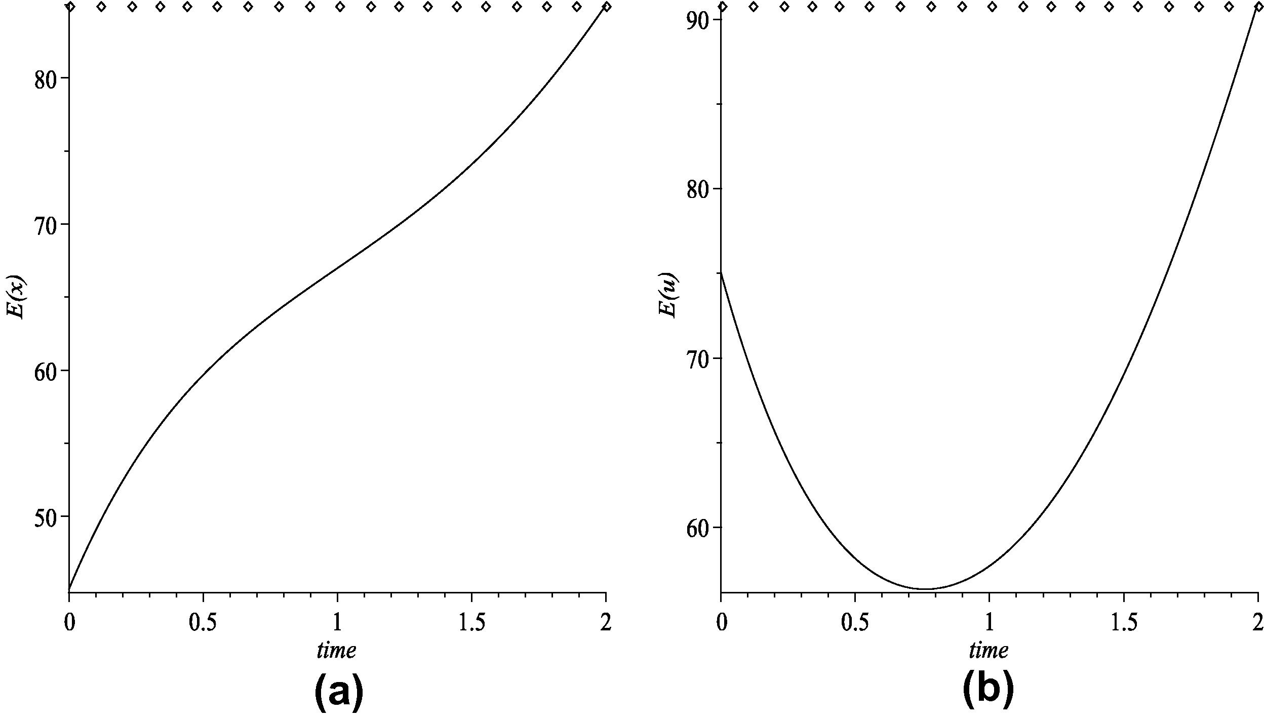
In this subsection, we draw the graph of time behavior of both of optimal expected inventory level and optimal expected production rate with a constant demand rate. In the this case, the following set of parameter values and initial state are adopted:

Parameter	E(x₀)	E(u₀)	x₁	u₁	h	c	θ	σ	T	k
Value	45	75	35	75	1.0	1.5	0.1	0.05	2.0	0.5

The numerical results are illustrated in Fig. 1a and b. We conclude that both of the optimal expected inventory level and the optimal expected production rate go to their goal values, respectively, at the end of time horizon.

(a) The optimal expected inventory level and (b) the optimal expected production rate.

4.2

4.2 Exponential time demand rate

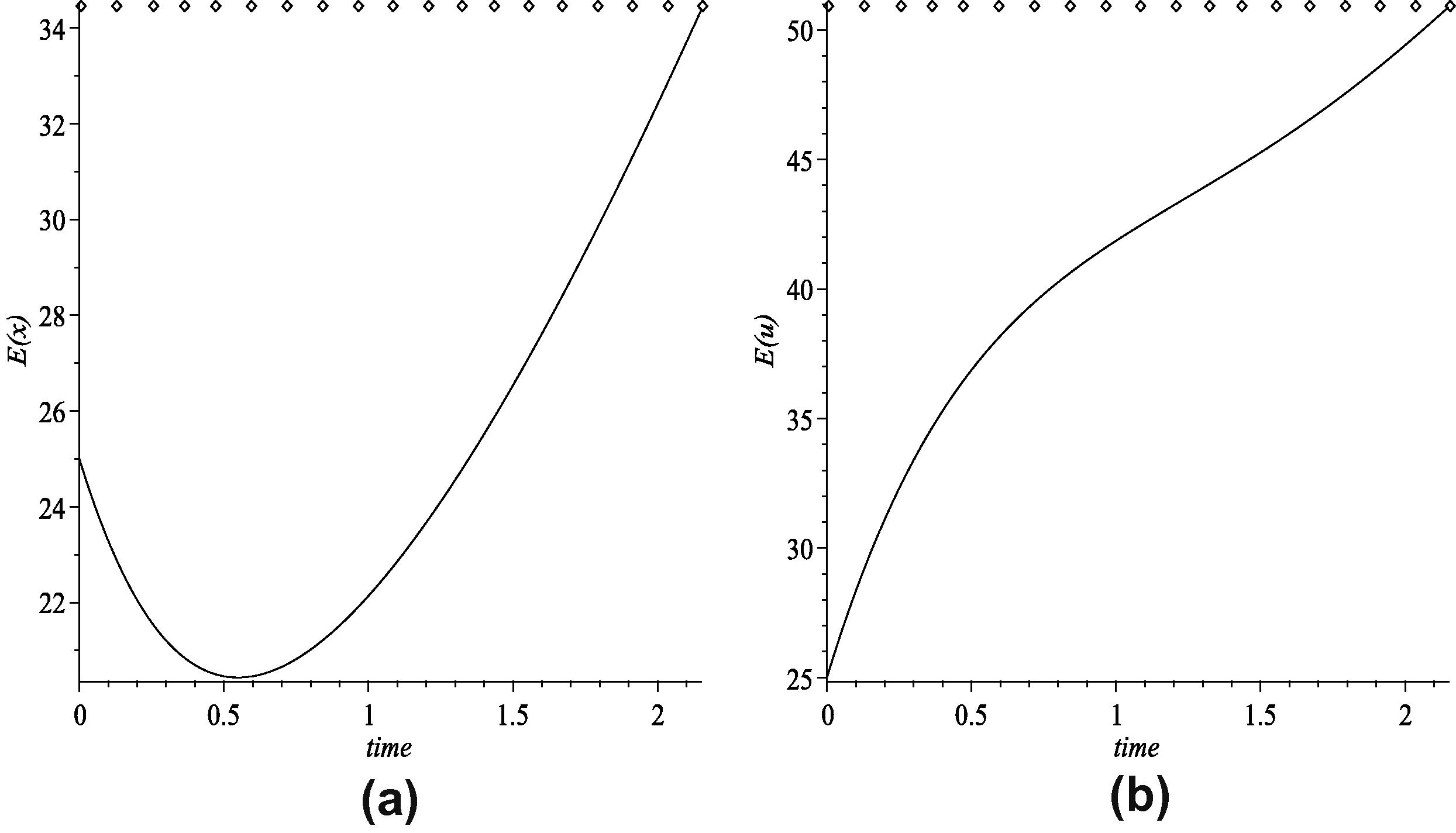
In this subsection, we draw of the graph of time behavior of both of optimal expected inventory level and optimal expected production rate with an exponential function of time demand rate. In this case, the following set of parameter values and initial state are adopted:

Parameter	E(x₀)	E(u₀)	x₁	u₁	h	c	θ	σ	T	k
Value	25	25	15	35	0.5	2.0	0.05	0.01	2.15	0.5

The numerical results are illustrated in Fig. 2a and b. We conclude that both of the optimal expected inventory level and the optimal expected production rate go to their goal values, respectively, at the end of time horizon.

4.3

4.3 Linear demand rate of expected inventory level

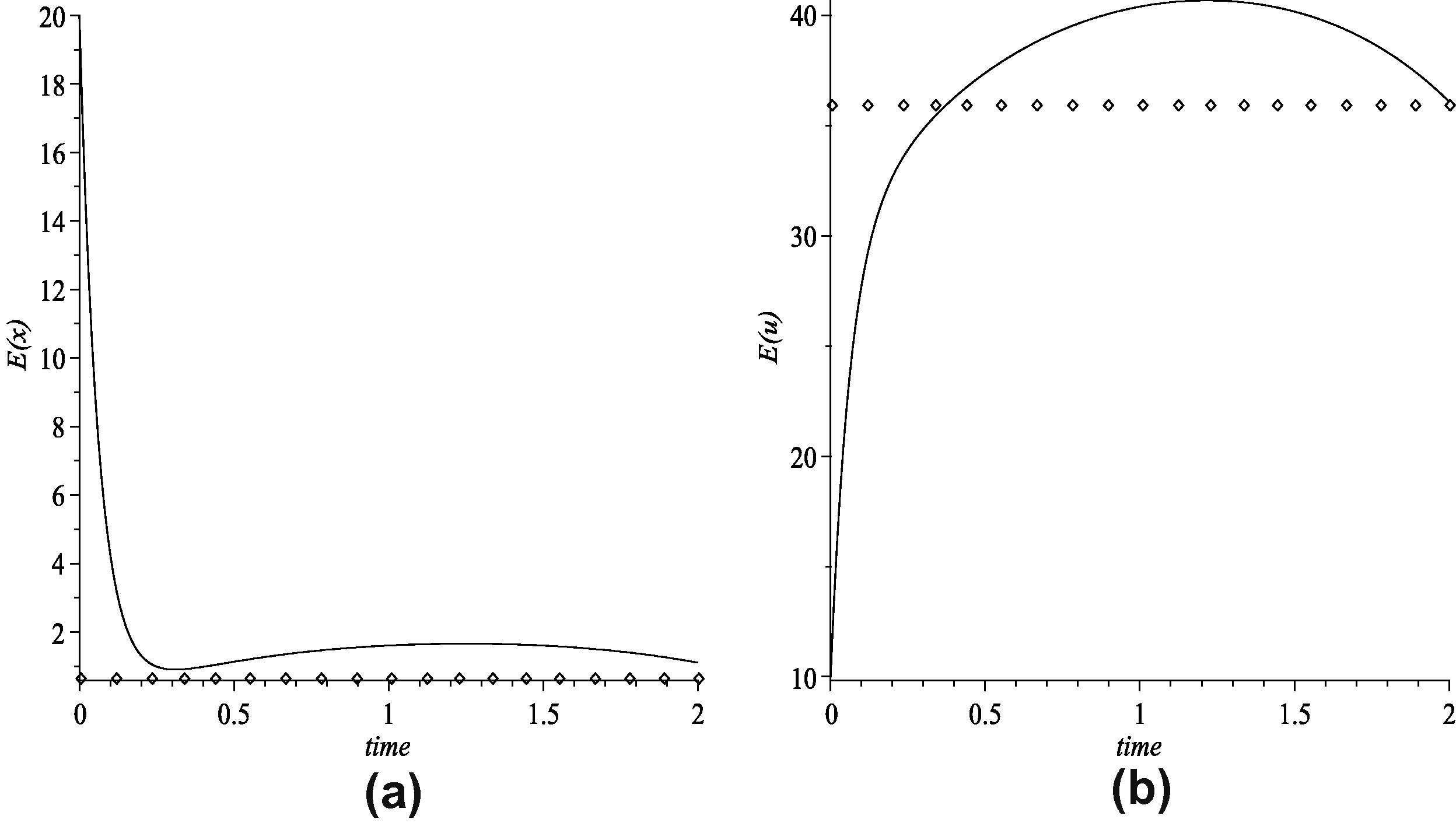
In this subsection, we draw the graph of the time behavior of both of optimal expected inventory level and optimal expected production rate when the demand rate is a linear function of optimal expected inventory level. In this example, the following set of parameter values and initial state is adopted:

Parameter	E(x₀)	E(u₀)	x₁	u₁	h	c	θ	σ	T	k
Value	20	10	20	45	0.75	2.0	0.05	0.01	2	15

The numerical results are illustrated in Fig. 3a and b. We conclude that both of the optimal expected inventory level and the optimal expected production rate go to their goal values, respectively, at the end of time horizon.

4.4

4.4 Logistic demand rate of expected inventory level

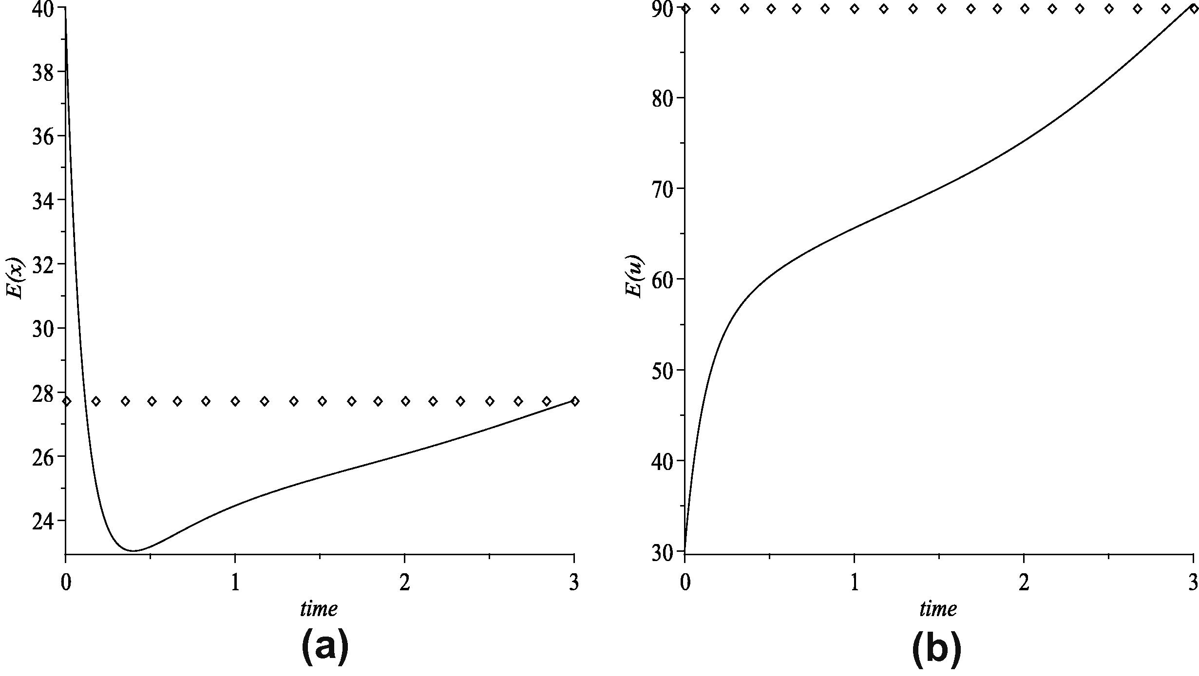
In this subsection, we draw the graph of the time behavior of both of optimal expected inventory level and optimal expected production rate when the demand rate is a logistic function of optimal expected inventory level. In this case, the following set of parameter values and initial state are adopted:

Parameter	E(x₀)	E(u₀)	x₁	u₁	h	c	θ	σ	T	B	k
Value	40	30	6	27.5	0.75	2.0	0.05	0.01	3	25	8

The numerical results are illustrated in Fig. 4a and b. We conclude that both of the optimal expected inventory level and the optimal expected production rate go to their goal values, respectively, at the end of time horizon.

5 Conclusion

We have shown in this paper how to use a stochastic control technique to optimize a production-inventory system subjected to perturbation noises that can be represented by a Wiener process. The paper used the Hamilton–Jacobi–Bellman principle to find the optimal expected inventory level and optimal expected production rate that minimize the current value of the expected holding and production costs for a stochastic production-inventory system. The paper generalizes some previous work in this field. This paper has discussed some special cases of demand rates. Numerical examples was analyzed for different cases of the demand rate.

References

Benkherouf L., Aggoun L., . On a stochastic inventory model with deterioration and stock-dependent demand items. Probability in the Engineering and Informational Sciences. 2002;16:151-165.
[Google Scholar]
Benkherouf L., Johnson M., . On a stochastic demand jump inventory model. Mathematical and Computer Modelling. 2009;50:1218-1228.
[Google Scholar]
Davis M.H., . Linear Estimation and Stochastic Control. New York: John Wiely & Sons; 1994.
El-Gohary A., . Optimal control of stochastic lattice of prey-predator models. Applied Mathematics and Computation. 2005;160:15-28.
[Google Scholar]
Goyal S.K., Giri B.C., . Recent trends in modeling of deteriorating inventory. European Journal of Operational Research. 2001;134:1-16.
[Google Scholar]
Kendrick D.A., . Stochastic control for economic models: past, present and the paths ahead. Journal of Economic Dynamics & Control. 2005;29:3-30.
[Google Scholar]
Kendrick D.A., Amman H.M., . A classification system for economic stochastic control models. Computational Economics. 2006;27:453-481.
[Google Scholar]
Kenné J.P., Gharbi A., . Stochastic optimal production control problem with corrective maintenance. Computers and Industrial Engineering. 2004;46:865-875.
[Google Scholar]
Parlar M., . A stochastic production planning model with a dynamic chance constraint. European Journal of Operational Research. 1985;20:255-260.
[Google Scholar]
Perkins J.R., Kumar P.R., . Optimal control of pull manufacturing systems. IEEE Transactions on Automatic Control. 1994;40:2040-2051.
[Google Scholar]
Presman E., Sethi S.P., . Inventory models with continuous and Poisson demands and discounted and average costs. Production and Operations Management. 2006;55:279-293.
[Google Scholar]
Sethi S.P., Thompson G.L., . Optimal Control Theory: Applications to Management Science and Economics (Second ed.). Dordrecht: Kluwer Academic Publishers; 2000.
Shen R.F.C., . Aggregate production planning by stochastic control. European Journal of Operational Research. 1994;73:346-359.
[Google Scholar]
Yang J., Yan H., Sethi S.P., . Optimal production planning in pull flow lines with multiple products. European Journal of Operational Research. 1999;119:582-604.
[Google Scholar]
Yin K., Liu H., Yin G., . Stochastic models and numerical solutions for production planning with applications to the paper industry. Computers and Chemical Engineering. 2003;27:1693-1706.
[Google Scholar]