Optimal analysis of adaptive type-II progressive censored for new unit-lindley model

Amani Alrumayh; Wajaree Weera; Hazar A. Khogeer; Ehab M. Almetwally

doi:10.1016/j.jksus.2022.102462

View/Download PDF

Optimal analysis of adaptive type-II progressive censored for new unit-lindley model

Amani Alrumayh^{^a}, Wajaree Weera^{^b,⁎}, Hazar A. Khogeer^{^c}, Ehab M. Almetwally^{^d,^e}

a Department of Mathematics, College of Science, Northern Border University, Arar, Saudi Arabia

b Department of Mathematics, Faculty of Science, Khon Kaen University, Khon Kaen 40002, Thailand

c Department of Mathematical Sciences, College of Applied Sciences, Umm Al-Qura University, Makkah, Saudi Arabia

d Faculty of Business Administration, Delta University of Science and Technology, Gamasa 11152, Egypt

e The Scientific Association for Studies and Applied Research, Al Manzalah 35646, Egypt

⁎Corresponding author at: Department of Mathematics, Faculty of Science, Khon Kaen University, Khon Kaen 40002, Thailand wajawe@kku.ac.th (Wajaree Weera),

Received: 2022-3-7, Accepted: 2022-11-18,

Disclaimer:
This article was originally published by Elsevier and was migrated to Scientific Scholar after the change of Publisher.

Peer review under responsibility of King Saud University.

Abstract

The parameters, reliability, and hazard rate functions of the Unit-Lindley distribution based on adaptive Type-II progressive censored sample are estimated using both non-Bayesian and Bayesian inference methods in this study. The Newton–Raphson method is used to obtain the maximum likelihood and maximum product of spacing estimators of unknown values in point estimation. On the basis of observable Fisher information data, estimated confidence ranges for unknown parameters and reliability characteristics are created using the delta approach and the frequentist estimators’ asymptotic normality approximation. To approximate confidence intervals, two bootstrap approaches are utilized. Using an independent gamma density prior, a Bayesian estimator for the squared-error loss is derived. The Metropolis–Hastings algorithm is proposed to approximate the Bayesian estimates and also to create the associated highest posterior density credible intervals. Extensive Monte Carlo simulation tests are carried out to evaluate the performance of the developed approaches. For selecting the optimum progressive censoring scheme, several optimality criteria are offered. A practical case based on COVID-19 data is used to demonstrate the applicability of the presented methodologies in real-life COVID-19 scenarios.

Keywords

Adaptive Type-II progressive censoring

Bayesian estimator

Bootstrapping

Metropolis-Hasting algorithm

Reliability

Unit-Lindley distribution

Show Related Articles from PubMed

1 Introduction

The life test finishes when the necessary effective sample is reached, thanks to adaptive Type-II progressive censoring. It also assures that the parametric inference and total duration test are both improved. Because many new goods have a long lifetime due to high manufacturing accuracy, obtaining failures is difficult with this high manufacturing technology, so we apply a censor scheme to decrease costs and time in lifetime studies. As a result, we require a suitable distribution capable of simulating failure times from censored experiments in this setting. As a result, we chose a really intriguing distribution for this investigation.

The one-parameter of New unit-Lindley (NUL) distribution was originally proposed by Mazucheli et al. (2019) by using transformation to the traditional Lindley distribution. But let’s say that the lifetime random variable X of a certain test item complies with $UL (θ)$ . We can use the following well known (CDF) abbreviations (CDF) is uesd for the cumulative distribution function, and (PDF) is used for probability density function, in the same way we express reliability function by RF, and the hazard rate function can be abbreviated by (HRF), and reversed HRF can be expressed by the abbreviation (RHRF), at different times t, are each supplied, are follows:

(1)

f (x; θ) = \frac{θ^{2}}{x^{3} (θ + 1)} e^{- θ \frac{1 - x}{x}}, 0 < x < 1, θ > 0,

(2)

F (x; θ) = \frac{θ + x}{x (1 + θ)} e^{- θ \frac{1 - x}{x}}, 0 < x < 1, θ > 0,

(3)

R (t; θ) = 1 - \frac{θ + t}{t (1 + θ)} e^{- θ \frac{1 - t}{t}}, 0 < t < 1, θ > 0,

(4)

hr (t; θ) = \frac{t^{- 2} θ^{2}}{t (1 + θ) e^{θ \frac{1 - t}{t}} - (θ + t)}, 0 < t < 1, θ > 0,

(5)

\begin{matrix} and \\ rhr (t; θ) = \frac{θ^{2}}{t^{2} (θ + t)}, & 0 < t < 1, θ > 0 . \end{matrix}

Also, Mazucheli et al. (2019) introduced the regression model of the NUL distribution as an alternative model of the unit-Lindley and beta regression. UL was discussed by Mazucheli et al. (2020) and is helpful for data processing in the [0,1] range. It has a few intriguing characteristics, such belonging to the exponential family and having closed form expressions for the moments. Nadarajah and Chan (2020) derived closed form expressions moments and incomplete moments of UL distribution. Irshad et al. (2021) considered an exponential version of UL distribution. Biswas and Chakraborty (2021) estimated the R = P (Y < X) for unit-Lindley distribution: inference with an application in public health. Furthermore, the NUL distribution has superior features in many practical scenarios and can be used to fit survival data when compared to these lifespan distributions. As a result, the NUL distribution may be a useful alternative for analysing skewed data that resembles these skewed distributions. Fig. 1 displays many representations of the NUL distribution’s density function as well as its failure rate function. using certain predetermined values within a set of the parameter called

θ

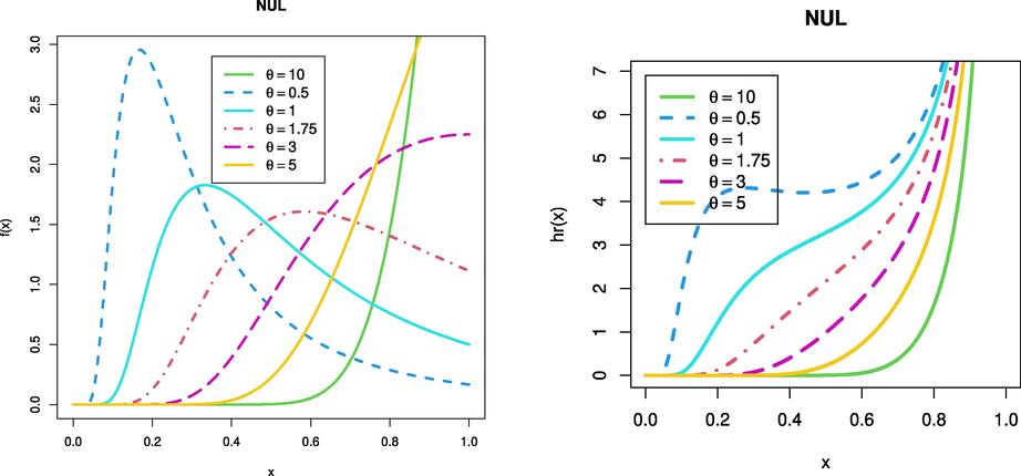
Plots of the density and hazard rate functions of the NUL distribution.

In the context of censoring mechanisms, in recent few years, several works considered various statistical inferences of the unknown Lindley parameters. Goel and Krishna (2020) developed the progressive type-II (PCS-T2) random censoring scheme with Lindley failure and censoring time distributions. Hafez et al. (2020) discussed Lindley distribution with accelerated life tests. Developments of Weibull distribution are discussed in many papers (Aslam et al., 2011; Aslam et al., 2017). For more reading about distribution theory see (Lin et al., 2021 (2021).; Zhou et al., 2021; Alsuhabi et al., 2022; Wang et al., 2022; Alkhairy et al., 2022 ).

The lifetime of some products has greatly increased as a result of improvements in digital transformation and industrial design and technology. Even with progressive filtering, the duration test takes a long time in this case, and there are occasionally no (or few) failures during the test. Ng et al. (2009) offered adaptive Type-II progressive censoring algorithms as a result (APCS-T2). We propose (Balakrishnan and Cramer, 2014) for more information on how prevalent this censoring method has grown in survival analysis and reliability research. Briefly, the APCS-T2 is stated as: Assume progressive censoring, effective sample size of $(m < n)$ , and n independent and identical units $(R_{1}, R_{2}, \dots, R_{m})$ , threshold time pointTsuch that $T \in (0, \infty)$ , are predetermined at the beginning of the experiment. According to (Ng et al., 2009), the APCS-T2 is a test that permits $R_{i}, i = 1, 2, \dots, m$ to change in the test and allows the experiment time to slightly exceed the stated period T. Because of this modification, the experimenter will be able to call off the study after the desired number of representative samples has been collected. Let $((X_{1 : m : n}, R_{1}), (X_{2 m : n}, R_{2}), \dots, (X_{m : m : n}, R_{m}))$ be a PCS-T2. If $X_{m : m : n} < T$ , then the experiment terminates at $X_{m : m : n}$ , which is just the usual PCS-T2. Otherwise, if $X_{d : m : n} < T < X_{d + 1 : m : n}$ , for $d = 1, 2, \dots, m - 1$ , (where dstands the number of the failures that take place before T) then the units sill under observation without any removals during the test, i.e., set $R_{i} = 0$ for $i = d + 1, \dots, m - 1$ and then removed the remaining surviving items at the time of observed $m^{th}$ failure, i.e., $R_{m}^{*} = n - m - \sum_{i = 1}^{d} R_{i}$ . However, let $\underset{̲}{x} = \{(X_{1 : m : n}, R_{1}), \dots, (X_{d : m : n}, R_{d}), (X_{d + 1 m : n}, R_{d + 1}), \dots, (X_{m : m : n}, R_{m})\}$ were an adaptive sample that is progressively Type-II censored and follows a continuous population, then the joint likelihood function of the APCS-T2 would look like this: where $\underset{̲}{θ}$ is interpreted to imply as below:

(6)

L (\underset{̲}{θ}| \underset{̲}{x}) = A_{d} \prod_{i = 1}^{m} f (x_{i : m : n}; \underset{̲}{θ}) \prod_{i = 1}^{d} {[\overline{F} (x_{i : m : n}; \underset{̲}{θ})]}^{R_{i}} {[\overline{F} (x_{m : m : n}; \underset{̲}{θ})]}^{R_{m}^{*}},

where

A_{d}

represents the constant used

\overline{F} (x_{i : m : n}; \underset{̲}{θ}) = 1 - F (x_{i : m : n}; \underset{̲}{θ})

and

R_{m}^{*} = n - m - \sum_{i = 1}^{d} R_{i}

In addition to the conventional likelihood function (LF) of APCS-T2 that is detailed in the previous sentence, the maximum product of spacing (MPS) technique is also taken into consideration to be a competitive way in (6). Cheng and Amin (1983) and Ranneby (1984) separately introduced and explored the PS technique as an alternate strategy for estimating parameter(s) of continuous univariate distributions. The maximum product spacing estimators methods (MPSEs) is comprehensively studied considering several cases as in Refs. (Anatolyev and Kosenok, 2005; Alshenawy et al., 2020; Alshenawy et al., 2021; Almetwally et al., 2023 ).

The APCS-T2 utilising the maximum PS approach, $S (\cdot)$ , can be defined as follows, according to (Almetwally et al., 2019; Almetwally et al., 2020; El-Sherpieny et al., 2020; Ahmad et al., 2022 ):

(7)

S (\underset{̲}{θ}| \underset{̲}{x}) = B_{d} \prod_{i = 1}^{m + 1} [F (x_{i : m : n}; \underset{̲}{θ}) - F (x_{i - 1 : m : n}; \underset{̲}{θ})] \prod_{i = 1}^{d} {[\overline{F} (x_{i : m : n}; \underset{̲}{θ})]}^{R_{i}} {[\overline{F} (x_{m : m : n}; \underset{̲}{θ})]}^{R_{m}^{*}},

where

B_{d}

represents the constant used,

F (x_{0 : m : n}; \underset{̲}{θ}) \equiv 0

and

F (x_{m + 1 : m : n}; \underset{̲}{θ}) \equiv 1

. Henceforward, we’ll use

x_{i}

instead of

x_{i : m : n}

for simplify notations. A schematic illustration of the APCS-T2 is depicted in Fig. 2.

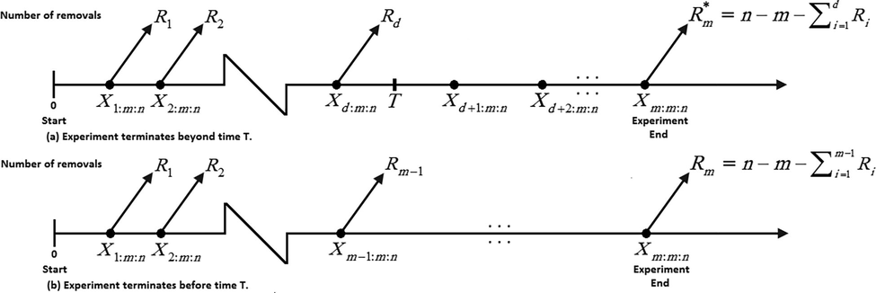
Schematic illustration of Type-II adaptive progressively censoring.

Many papers discussed different points of COVID-19 data using several methods, such as: amma-distributed variables by Aslam et al. (2021), neutrosophic statistics by Sherwani et al. (2021), repetitive sampling under indeterminacy by Rao and Aslam (2021), and modeling to Factor Productivity of the United Kingdom by Alyami et al. (2022).

To our knowledge, no work has been published on applying adaptive Type-II progressive hybrid censoring to infer the NUL distribution’s model parameters and/or reliability traits, such as R and HRF, which is more significant in a range of real-world contexts. As a result, in this study, we will exclusively focus on both classical and Bayesian estimating methodologies to generate point and interval estimates of unknown model parameters, as well as some life parameters of the HD under APCS-T2, such as RF and HRF. In this paper, LF and MPS procedures, as well as the Bayesian estimate method, are applied. We estimated the (ACIs) of the NUL parameter are produced using the delta approach.

Using independent gamma priors, the likelihood function under squared-error loss (SEL) produces the Bayes estimate of the unknown parameter. The Bayes estimators and related credible ranges cannot be solved analytically, hence Markov chain Monte Carlo (MCMC) techniques are employed to create samples from the relevant posterior density functions. Finding the optimum censorship scheme from a collection of all conceivable removal patterns that provide a plethora of information about the unknown model parameter in issue is one of the most challenging tasks in dependability research. This is one of the most difficult aspects of the research process. One real data set of COVID-19 is investigated to illustrate the suggested methodologies’ application to real-world phenomena and to highlight the NUL distribution’s superiority. Finally, we formulate some particular suggestions based on the numerical data.

The remainder of the work in the paper is structured as follows: The traditional estimate of an unknowable parameter, in addition to the features of dependability, is presented here in Section 2. In Section 3, we begin the process of developing the Bayesian estimate based on the SEL function utilising each of the provided frequentist functions. In Section 4, The most optimal ideas for progressive censorship are discussed here. Section 5 presents the simulated findings. In Section 6 an optimal censoring strategy is also suggested along with a real data analysis that, which is offered for demonstrative purposes. Finally, we include the paper’s main findings in Section 7.

2 Classical inference

Using data collected using the suggested censoring approach, this section will employ the LF and MPS procedures to generate point and interval estimators for the unknown parameters, as well as the reliability aspects of the NUL distribution. Prior to proceeding, let us assume that $X_{1} < \dots < X_{d} < T < X_{d + 1} < \dots < X_{m}$ is an APCS-T2 censored order statistics of size $m (< n)$ with censoring scheme $R_{1}, \dots, R_{d}, 0, \dots, 0, n - m - \sum_{i = 1}^{d} R_{i}$ from $NUL (θ)$ .

2.1

2.1 Maximum likelihood estimator

Without taking into account any additive constants, (2) and (1) are substituted into the likelihood function (6) to produce

(8)

L (θ| \underset{̲}{x}) \propto \frac{θ^{2 m}}{{(θ + 1)}^{m}} {(ξ (x_{m}; θ))}^{R_{m}^{*}} e^{- θ \sum_{i = 1}^{m} \frac{1 - x_{i}}{x_{i}}} \prod_{i = 1}^{m} x_{i}^{- 3} \prod_{i = 1}^{d} {(ξ (x_{i}; θ))}^{R_{i}},

where

ξ (t; θ) = 1 - \frac{θ + t}{t (1 + θ)} e^{- θ \frac{1 - t}{t}}

The related log-likelihood function for (8) is $ℓ (\cdot) = \log L (\cdot)$ .

(9)

ℓ (θ| d) = 2 m \ln (θ) - m \ln (θ + 1) + R_{m}^{*} \ln (ξ (x_{m}; θ)) - θ \sum_{i = 1}^{m} \frac{1 - x_{i}}{x_{i}} - 3 \sum_{i = 1}^{m} \ln (x) + R_{i} \sum_{i = 1}^{d} \ln (ξ (x_{i}; θ)) .

Differentiating (9) partially with respect to the parameter $θ$ then equate (10) to zero, as below we can get the equation:

(10)

\frac{\partial ℓ}{\partial θ} = \frac{2 m}{θ} - \frac{m}{θ + 1} + R_{m}^{*} \frac{ξ^{'} (x_{m}; θ)}{ξ (x_{m}; θ)} - \sum_{i = 1}^{m} \frac{1 - x_{i}}{x_{i}} + R_{i} \sum_{i = 1}^{d} \frac{ξ^{'} (x_{i}; θ)}{ξ (x_{i}; θ)},

where

ξ_{θ}^{'} (t; θ) = [\frac{1 - t}{t} \frac{θ + t}{t (1 + θ)} - \frac{(1 - t)}{t {(1 + θ)}^{2}}] e^{- θ \frac{1 - t}{t}}

As it seems, from (10), analytic solution of MLE of $θ$ is not available. As a result, the ”maxLik” package may be used numerically to create an iterative Newton Raphson (NR) approach to get the desired MLE $\hat{θ}$ for any given data set. Once the maximum likelihood estimate of $θ$ calculated, the MLE of the reliability indices $RF (t)$ (3) and $HRF (t)$ (4) at any mission time $0 < t < 0$ can be easily derived using the invariance property of MLE $\hat{θ}$ as $\hat{R} (t) = 1 - \frac{\hat{θ} + t}{t (1 + \hat{θ})} e^{- \hat{θ} \frac{1 - t}{t}}, 0 < t < 0, and \hat{hr} (t) = \frac{t^{- 2} {\hat{θ}}^{2}}{t (1 + \hat{θ}) e^{\hat{θ} \frac{1 - t}{t}} - (\hat{θ} + t)}, 0 < t < 0 .$

2.2

2.2 Maximum product of spacings estimators

Substituting (2) and (1) into (7), the product of spacings (7) becomes

(11)

S (θ| \underset{̲}{x}) \propto {[ξ (x_{m}; θ)]}^{R_{m}^{*}} \prod_{i = 1}^{m + 1} [\frac{θ + x_{i}}{x_{i} (1 + θ)} e^{- θ \frac{1 - x_{i}}{x_{i}}} - \frac{θ + x_{i - 1}}{x_{i - 1} (1 + θ)} e^{- θ \frac{1 - x_{i - 1}}{x_{i - 1}}}] \prod_{i = 1}^{d} {(ξ (x_{i}; θ))}^{R_{i}} .

From (11), the MPSE $\hat{θ}$ of $θ$ , may be accomplished by raising the value of the log-PS function in the following, $s (\cdot) \propto \log S (\cdot)$ , as

(12)

s (θ| \underset{̲}{x}) \propto R_{m}^{*} \ln [ξ (x_{m}; θ)] + \sum_{i = 1}^{m + 1} \ln [\frac{θ + x_{i}}{x_{i} (1 + θ)} e^{- θ \frac{1 - x_{i}}{x_{i}}} - \frac{θ + x_{i - 1}}{x_{i - 1} (1 + θ)} e^{- θ \frac{1 - x_{i - 1}}{x_{i - 1}}}] + R_{i} \sum_{i = 1}^{d} \ln (ξ (x_{i}; θ)) .

Differentiating (12) partially in respect of $θ$ , we have two nonlinear equation that must be solved simultaneously to obtain respective $\hat{θ}$ as

(13)

\frac{\partial s}{\partial θ} = R_{m}^{*} \frac{ξ^{'} (x_{m}; θ)}{ξ (x_{m}; θ)} + \sum_{i = 1}^{m + 1} \frac{ξ^{'} (x_{i - 1}; θ) - ξ^{'} (x_{i}; θ)}{\frac{θ + x_{i}}{x_{i} (1 + θ)} e^{- θ \frac{1 - x_{i}}{x_{i}}} - \frac{θ + x_{i - 1}}{x_{i - 1} (1 + θ)} e^{- θ \frac{1 - x_{i - 1}}{x_{i - 1}}}} + R_{i} \sum_{i = 1}^{d} \frac{ξ^{'} (x_{i}; θ)}{ξ (x_{i}; θ)},

The MPSE lacks an explicit form, just like the MLE. As a result, the NR approach is employed to quantitatively determine the MPSE from (13) for a simulation or particular datasets. Cheng and Amin (1983) proved that MPSE is a superior method of estimation. Since the MPSE possess the invariance principle similar to the MLE, the MPSE $\hat{RF} (t)$ and $\hat{h} (t)$ of $RF (t)$ and $HRF (t)$ can be easily obtained by replacing the unknown parameters $θ$ in (10) by their $\hat{θ}$ , respectively, as $\hat{R} (t) = 1 - \frac{\hat{θ} + t}{t (1 + \hat{θ})} e^{- \hat{θ} \frac{1 - t}{t}}, 0 < t < 0, and \hat{hr} (t) = \frac{t^{- 2} {\hat{θ}}^{2}}{t (1 + \hat{θ}) e^{\hat{θ} \frac{1 - t}{t}} - (\hat{θ} + t)}, 0 < t < 0 .$

2.3

2.3 Asymptotic confidence intervals

In this section we used the Fisher’s information matrix $I (θ) = E [- (\partial^{2} ℓ (θ| \underset{̲}{x})) / \partial θ^{2}]$ to get the ACIs. The asymptotic variance covariance (VarCov) matrix of the MLE $\hat{θ}$ can be produced by inverting $I (\underset{̲}{θ})$ and removing Ewith replacing $θ$ by their MLE $\hat{θ}$ , as shown in Lawless (Lawless, 2003). This is due to the fact that obtaining exact results to Fisher’s expectation is a time-consuming process. Also, (Anatolyev and Kosenok, 2005) stated that the MLE $\hat{ω}$ and MPSE $\hat{ω}$ are asymptotically analogous, in fact, $\hat{ω} = \hat{ω} + o (n^{- 1 / 2})$ .

The approximate VarCov matrix, $I^{- 1} (\hat{θ})$ , can be expressed so easily as follows:

(14)

I^{- 1} (\hat{θ}) = {[\begin{matrix} - \end{matrix} ℓ_{11}]}_{\hat{θ}}^{- 1} = [\begin{matrix} {\hat{σ}}_{\hat{θ} \hat{θ}} \end{matrix}] .

In a similar manner, by finding the derivative of (12) at their MPSE $\hat{θ}$ , the approximate V-C matrix, $I^{- 1} (\hat{θ})$ , is provided through the following equation

(15)

I^{- 1} (\hat{θ}) = {[\begin{matrix} - \end{matrix} s_{11}]}_{\hat{θ}}^{- 1} = [\begin{matrix} {\hat{σ}}_{\hat{θ} \hat{θ}} \end{matrix}] .

The Fisher’s element as in (14) and (15) are obtained and provided as following:

(16)

\frac{\partial^{2} ℓ}{\partial θ^{2}} = \frac{- 2 m}{θ^{2}} - \frac{- m}{{(θ + 1)}^{2}} + R_{m}^{*} \frac{ξ^{″} (x_{m}; θ) ξ (x_{m}; θ) - ξ^{' 2} (x_{m}; θ)}{ξ^{2} (x_{m}; θ)} + R_{i} \sum_{i = 1}^{d} \frac{ξ^{″} (x_{m}; θ) ξ (x_{m}; θ) - ξ^{' 2} (x_{m}; θ)}{ξ^{2} (x_{m}; θ)},

and

(17)

\begin{matrix} \frac{\partial^{2} s}{\partial θ^{2}} = & R_{m}^{*} \frac{ξ^{″} (x_{m}; θ) ξ (x_{m}; θ) - ξ^{' 2} (x_{m}; θ)}{ξ^{2} (x_{m}; θ)} + \sum_{i = 1}^{m + 1} \frac{η (x_{i}; θ) [ξ^{″} (x_{i - 1}; θ) - ξ^{″} (x_{i}; θ)]}{{[\frac{θ + x_{i}}{x_{i} (1 + θ)} e^{- θ \frac{1 - x_{i}}{x_{i}}} - \frac{θ + x_{i - 1}}{x_{i - 1} (1 + θ)} e^{- θ \frac{1 - x_{i - 1}}{x_{i - 1}}}]}^{2}} \\ + \sum_{i = 1}^{m + 1} \frac{{[ξ^{'} (x_{i - 1}; θ) - ξ^{'} (x_{i}; θ)]}^{2}}{{[η (x_{i}; θ)]}^{2}} + R_{i} \sum_{i = 1}^{d} \frac{ξ^{″} (x_{i}; θ) ξ (x_{i}; θ) - ξ^{' 2} (x_{i}; θ)}{ξ^{2} (x_{i}; θ)}, \end{matrix}

where

η (x_{i}; θ) = \frac{θ + x_{i}}{x_{i} (1 + θ)} e^{- θ \frac{1 - x_{i}}{x_{i}}} - \frac{θ + x_{i - 1}}{x_{i - 1} (1 + θ)} e^{- θ \frac{1 - x_{i - 1}}{x_{i - 1}}}

The estimated variances of $R (t)$ and $hr (t)$ must be obtained before the ACIs of $R (t)$ and $hr (t)$ can be constructed. The delta approach is the most statistically efficient method for constructing confidence intervals in practice. This approach is more beneficial and simple to apply than the empirically-driven bootstrap approach, which should only be used as a last resort when the Taylor series approximation is empirically inaccurate see (Greene, 2000). However, based on the asymptotic normality of the MLEs of the reliability parameters of life $R (t)$ and $h (t)$ , we have $\hat{R} (t) \sim N (\hat{R} (t), σ_{\hat{R} (t)}^{2})$ and $\hat{hr} (t) \sim N (\hat{hr} (t), σ_{\hat{h} (t)}^{2})$ . According to the delta method, from (14), the ACIs for $R (t)$ and $hr (t)$ can be constructed using the corresponding normality, respectively as ${\hat{σ}}_{\hat{R} (t)}^{2} = [Δ_{R (t)} I^{- 1} (θ) Δ_{R (t)}^{T}] |_{(\hat{θ})}, and {\hat{σ}}_{\hat{hr} (t)}^{2} = [Δ_{hr (t)} I^{- 1} (θ) Δ_{hr (t)}^{T}] |_{(\hat{θ})},$ where $Δ_{R (t)}$ and $Δ_{h (t)}$ are the gradient of $R (t)$ and $hr (t)$ obtained at $\hat{θ}$ as $Δ_{R (t)} = [\partial R (t) / \partial θ], and Δ_{hr (t)} = [\partial hr (t) / \partial θ] .$

Hence, using the concept of large sample theory for MLE $\hat{ω}$ of $ω$ , the $100 (1 - γ) %$ two-sided ACIs for the unknown parameter $θ, R (t)$ or $hr (t)$ is given by $\hat{ω} \mp z_{γ / 2} \sqrt{{\hat{σ}}_{\hat{ω}}^{2}},$ where ${\hat{σ}}_{\hat{ω}}^{2}$ is the estimated variance of $\hat{ω}$ , and $z_{γ / 2}$ is the percentile of the standard normal distribution with upper probability $(γ / 2) - th$ .

In a similar pattern, from (15), the associated variance of $\hat{R} (t)$ and $\hat{hr} (t)$ obtained at their MPSE $\hat{θ}$ can be easily approximated and then the $100 (1 - γ) %$ ACIs of $ω$ using their MPSE $\hat{ω}$ can be easily constructed.

3 Bayesian estimators

Bayesian inference has risen to prominence in a variety of sectors, including but not limited to engineering, biology, clinical medicine, and so on. Its capacity to use prior information in the analysis makes it particularly valuable in dependability studies, where one of the major obstacles is data availability. The reliability parameters $R (t)$ and $hr (t)$ , as well as the Bayes estimates and related credible intervals of the model parameter $θ$ , are developed in this section.

3.1

3.1 Prior information and loss function

Using independent gamma priors is an easy approach that can result in findings with more explicit posterior density expressions because the gamma distribution can have a range of shapes based on its parameter values. As a result, we investigated the gamma density prior, which is more adjustable in terms of altering support for the NUL distribution parameter than more difficult prior distributions. As a result, it is believed that the NUL parameter $θ$ has independent gamma PDFs in the form of $Gamma (a, b)$ . The joint prior density of $θ$ then changes

(18)

π (θ) \propto θ^{a - 1} e^{- b θ}, θ > 0,

where the hyper-parameters

a, b

are selected to reflect prior information regarding the unknown parameter

θ

, and they are believed to be known and non-negative.

The choice of the symmetric loss function is a key issue in Bayesian analysis, according to the literature. The most often employed symmetric loss function in this study for estimating the considered unknown quantities is the SEL function, $L (\cdot)$ , which is defined as:

(19)

L (θ, \tilde{θ}) = {(\tilde{θ} - θ)}^{2},

where

\tilde{θ}

being an estimate of

θ

. Under (19), objective estimate

\tilde{θ}

is given by the posterior mean of

θ

. However, any other loss function can be easily incorporated.

3.2

3.2 Posterior analysis by LF

We can easily express the posterior PDF $π_{L} (\cdot)$ of $θ$ as shown below

(20)

π_{L} (θ| \underset{̲}{x}) = K_{1}^{- 1} π (θ) L (θ| \underset{̲}{x}),

where

K_{1} = \int_{0}^{\infty} π_{L} (θ| \underset{̲}{x}) d θ

is the normalizing constant.

The joint posterior PDF of $θ$ is obtained by substituting (8) and (18) into (20) as follows

(21)

π_{L} (θ| \underset{̲}{x}) = K_{1}^{- 1} \frac{θ^{2 m + a - 1}}{{(θ + 1)}^{m}} {(ξ (x_{m}; θ))}^{R_{m}^{*}} e^{- θ (b + \sum_{i = 1}^{m} \frac{1 - x_{i}}{x_{i}})} \prod_{i = 1}^{m} x_{i}^{- 3} \prod_{i = 1}^{d} {(ξ (x_{i}; θ))}^{R_{i}} .

The posterior expectation of $θ$ is the Bayes estimator for function of $θ$ under SEL function (19). Therefore, the marginal posterior distribution for $θ$ must be acquired in order to develop these estimations. In spite of this, it is plainly evident that it is not possible to get exact representations for the marginal PDF for unknown parameter $θ$ as a consequence of unstated mathematical terms of (21). We found a very flexible solution which is the MCMC approaches. In addition, in order to get the Bayesian estimates as well as the credible intervals that accompany them.

It is abundantly clear that the posterior distribution of $θ$ is incapable of being analytically converted to any well-known distribution, and as a result, it is not possible to sample it immediately using approaches that are commonplace. Therefore, it is suggested to simulate samples from (21) using the Metropolis Hastings (MH) algorithm with normal proposal distributions. Theta’s conditional PDFs’ diagram plot demonstrates how this distribution behaves similarly to the normal distribution.

As expect, similar to the case of Bayesian inference using LF approach, the posterior distribution (21) of $θ$ , is very hard to be represented using a specific known distribution. In order to approximate the Bayes estimates estimate of $θ, R (t), and$ hr(t), we thus consider using MCMC simulation technique.

The MH technique is a very useful MCMC strategy since it can generate random samples from a posterior density distribution with an independent proposal distribution, as well as calculate Bayes estimates and generate HPD credible intervals. Furthermore, this technique provides an easy-to-apply chain form of the Bayesian estimate from a practical standpoint. Please see (Gelman et al., 2004 and Lynch, 2007) for further information on this algorithm. The procedures that are outlined below need to be carried out in order to successfully produce random samples by using the assist MH algorithm.

Algorithm 1

We used the MH algorithm generate failure times that follows the NUL distribution to estimate the NUL parameter:

Step 1: Start with initial guess

(θ^{(0)}) = (\hat{θ})

Step 2: Set

j = 1

Step 3: Generate

θ^{*}

from (21) with normal distributions

N (\hat{θ}, σ_{\hat{θ} \hat{θ}})

, as

(a) Calculate

θ_{1} = \frac{π_{L} (θ^{*}| \underset{̲}{x})}{π_{L} (θ^{(j - 1)}| \underset{̲}{x})}

(b) Obtain

Q_{θ} = \min \{1, θ_{1}\}

u_{1}

and

u_{2}

from the uniform

U (0, 1)

distribution.

(d) If

u_{1} ⩽ Q_{θ}

, set

θ^{(j)} = θ^{*}

, else set

θ^{(j)} = θ^{(j - 1)}

Step 4: Compute the RF (3) and HRF (4), for a given distinct time

0 < t < 1

, as

R^{(j)} (t) = 1 - \frac{θ^{(j)} + t}{t (1 + θ^{(j)})} e^{- θ^{(j)} \frac{1 - t}{t}},

and

{hr}^{(j)} (t) = \frac{t^{- 2} {θ^{(j)}}^{2}}{t (1 + θ^{(j)}) e^{θ^{(j)} \frac{1 - t}{t}} - (θ^{(j)} + t)} .

Step 5: Set

j = j + 1

Step 6: Redo steps 2–5 for

N

times to collect

N

draws of

θ, R (t)

and

hr (t)

ω^{(j)} = (θ^{(j)}, R^{(j)} (t), h^{(j)} (t)), j = 1, 2, \dots, N .

Now, to construct the HPD credible interval of

θ

or the reliability characteristics

R (t)

and

hr (t)

, the associated simulated MCMC variates

ω^{(j)} = (θ^{(j)}, R^{(j)} (t), h^{(j)} (t))

for

j = N_{0} + 1, \dots, N

must be ordered as

ω_{(N_{0} + 1)}, ω_{(N_{0} + 2)}, \dots, ω_{(N)}

So by refering to (Chen and Shao, 1999), We can easily obtain the credible interval. $[ω_{(j^{*})}, ω_{(j^{*} + (1 - γ) (N - N_{0}))}],$ where $j^{*}$ is selected in such a way that $ω_{(j^{*} + \{(1 - γ) (N - N_{0})\})} - ω_{(j^{*})} = \min_{1 ⩽ j ⩽ γ (N - N_{0})} (ω_{(j + \{(1 - γ) (N - N_{0})\})} - ω_{(j)}), j^{*} = N_{0} + 1, N_{0} + 2, \dots, N .$

4 Optimum progressive censoring plans

When samples are acquired via censoring, we need an optimal plane, the preceding sections dealt with estimation methods of some lifetime parameters of $NUL (θ)$ . As an experimenter, you may want to choose the ‘optimal’ censoring scheme from the set of all possible options so that you may get the most out of your research. Choosing the best censoring strategy has been discussed in a variety of contexts in the past. However, a variety of optimality criteria and results on optimal censoring systems have been presented, see (Balakrishnan and Aggarwala, 2000).

Following (Ng et al., 2004), when the values of n(total test units), m(effective sample) and T is the time where the experiment is terminated, we can determine the optimal censoring design ( $R_{1}, R_{2}, \dots, R_{m}$ where $\sum_{i = 1}^{m} R_{i} = n - m$ ) under generalized Type-II progressively hybrid censored NUL model. several authors worked on the optimality planes, see for example, (Pradhan and Kundu, 2013). However, in order to develop the optimal PCS-T2 plan, many regularly utilised factors are taken into account, as mentioned in Table 5.

Regarding to criteria OA, our goal is minimization the determinant and trace of the VarCov matrix, while our goal regarding to criterion OCis maximization the main diagonal elements of the Fisher’s matrix $I (θ)$ , with respect to MLE $\hat{θ}$ , respectively. OAis $Minimize (I^{- 1} (\hat{θ}))$ and OC is $Maximize (I^{} (\hat{θ}))$ .

With reference to the OAcriterion, the goal that we have set for ourselves is to reduce the value of the VarCov matrices $I^{- 1} (\hat{φ})$ with respect to MLEs $\hat{φ}$ and MPSEs $\hat{φ}$ , respectively. In a similar vein, in terms of the criteria OC, improve the Fisher information matrices as much as possible $I (\hat{φ})$ and $I (\hat{φ})$ with respect to MLEs $\hat{φ}$ and MPSEs $\hat{φ}$ , respectively. The censoring plan that has been optimised to offer the most information corresponds to the optimality criteria that have the lowest value for the OAoptimality criterion and the greatest value for the OCoptimality criterion.

5 Generating simulated data data for estimation purpose

In this part we made a simulation experiment to asses the various estimation techniques, on the basis of adaptive Type-II progressive samples collected using a variety of methods for censoring.

5.1

5.1 Simulation purpose

Several simulation experiments were carried out to evaluate the performance of various item parameter estimation methodologies based on different schemes. The majority of studies, on the other hand, concentrated on likelihood estimation, product spacing, and Bayesian estimation. In addition, simulation research compares the efficacy of likelihood and product spacing estimation approaches to traditional estimation methods. Furthermore, sample size, censored adaptive time (t), censored progressive size (m), and censored sample schemes are all changed in a methodical manner. For the simulated data sets, the multiple methods indicated in Sections 2 and 3 were employed to estimate model parameters. To acquire the appropriate MLE and MPS, the iterative NR approach can be numerically implemented using the’maxLik’ package. Using an approximation normal distribution, the asymptotic confidence intervals were calculated. The MH method was used in order to generate Bayesian estimators that were dependent on the gamma prior.

For each predicted model parameter, the Bias (BS), mean square error (ME), and length of confidence intervals (LCONF) were calculated. The results of several schemes for estimating point parameters are shown in Tables 1–4 . Table 5 illustrate the results of various strategies for optimal censoring scheme. Tables 1–4 present the findings, which include some intriguing data.

Table 1 Results of simulation using classical and Bayesian methods, when the value of

θ = 0.5

n = 30.

	$θ$ =0.5			MLE			MPS			Bayesiam
m	scheme	T		BS	ME	LCONF	BS	ME	LCONF	BS	ME	LCONF
20	I	0.5	$θ$	0.0133	0.0057	0.2908	−0.0042	0.0051	0.2974	0.0144	0.0019	0.1528
			$R (T)$	0.0073	0.0016	0.1561	−0.0020	0.0015	0.1594	0.0078	0.0006	0.0824
			$hr (T)$	−0.0255	0.0233	0.5900	0.0102	0.0213	0.5356	−0.0290	0.0080	0.3107
		0.8	$θ$	0.0075	0.0048	0.2705	−0.0097	0.0045	0.2772	0.0078	0.0018	0.1557
			$R (T)$	0.0013	0.0001	0.0387	−0.0011	0.0001	0.0391	0.0012	0.0000	0.0220
			$hr (T)$	−0.0058	0.0031	0.2169	0.0079	0.0029	0.1951	−0.0062	0.0012	0.1251
	II	0.5	$θ$	0.0109	0.0064	0.3102	−0.0106	0.0058	0.3184	0.0156	0.0025	0.1654
			$R (T)$	0.0060	0.0018	0.1662	−0.0054	0.0017	0.1703	0.0085	0.0007	0.0891
			$hr (T)$	−0.0203	0.0260	0.6279	0.0236	0.0244	0.5616	−0.0312	0.0101	0.3369
		0.8	$θ$	0.0102	0.0056	0.2911	−0.0114	0.0051	0.2987	0.0098	0.0025	0.1864
			$R (T)$	0.0018	0.0001	0.0417	−0.0013	0.0001	0.0420	0.0015	0.0001	0.0265
			$hr (T)$	−0.0080	0.0036	0.2334	0.0093	0.0033	0.2052	−0.0078	0.0016	0.1496
	III	0.5	$θ$	0.0078	0.0048	0.2709	−0.0112	0.0045	0.2794	0.0114	0.0016	0.1426
			$R (T)$	0.0044	0.0014	0.1454	−0.0058	0.0013	0.1496	0.0062	0.0005	0.0768
			$hr (T)$	−0.0144	0.0200	0.5513	0.0245	0.0191	0.4943	−0.0230	0.0066	0.2912
		0.8	$θ$	0.0122	0.0055	0.2879	−0.0070	0.0050	0.2948	0.0116	0.0024	0.1748
			$R (T)$	0.0020	0.0001	0.0415	−0.0007	0.0001	0.0419	0.0018	0.0001	0.0249
			$hr (T)$	−0.0097	0.0036	0.2306	0.0058	0.0032	0.2056	−0.0092	0.0015	0.1403
25	I	0.5	$θ$	0.0094	0.0048	0.2703	−0.0077	0.0045	0.2778	0.0118	0.0017	0.1397
			$R (T)$	0.0052	0.0014	0.1452	−0.0040	0.0013	0.1489	0.0064	0.0005	0.0753
			$hr (T)$	−0.0177	0.0199	0.5485	0.0172	0.0187	0.4970	−0.0237	0.0068	0.2850
		0.8	$θ$	0.0106	0.0051	0.2775	−0.0066	0.0047	0.2847	0.0082	0.0019	0.1558
			$R (T)$	0.0018	0.0001	0.0401	−0.0007	0.0001	0.0405	0.0013	0.0000	0.0222
			$hr (T)$	−0.0083	0.0033	0.2223	0.0055	0.0030	0.2008	−0.0065	0.0012	0.1251
	II	0.5	$θ$	0.0094	0.0048	0.2703	−0.0077	0.0045	0.2778	0.0118	0.0017	0.1397
			$R (T)$	0.0052	0.0014	0.1452	−0.0040	0.0013	0.1489	0.0064	0.0005	0.0753
			$hr (T)$	−0.0177	0.0199	0.5485	0.0172	0.0187	0.4970	−0.0237	0.0068	0.2850
		0.8	$θ$	0.0106	0.0051	0.2775	−0.0066	0.0047	0.2847	0.0082	0.0019	0.1558
			$R (T)$	0.0018	0.0001	0.0401	−0.0007	0.0001	0.0405	0.0013	0.0000	0.0222
			$hr (T)$	−0.0083	0.0033	0.2223	0.0055	0.0030	0.2008	−0.0065	0.0012	0.1251
	III	0.5	$θ$	0.0030	0.0050	0.2781	−0.0146	0.0049	0.2854	0.0089	0.0016	0.1370
			$R (T)$	0.0018	0.0014	0.1491	−0.0076	0.0014	0.1528	0.0049	0.0005	0.0738
			$hr (T)$	−0.0045	0.0208	0.5653	0.0314	0.0205	0.5118	−0.0178	0.0065	0.2801
		0.8	$θ$	0.0064	0.0048	0.2719	−0.0113	0.0046	0.2794	0.0080	0.0021	0.1679
			$R (T)$	0.0012	0.0001	0.0390	−0.0013	0.0001	0.0395	0.0013	0.0000	0.0239
			$hr (T)$	−0.0050	0.0031	0.2180	0.0092	0.0030	0.1960	−0.0064	0.0014	0.1348

Table 2 Results of simulation using classical and Bayesian methods, when the value of

θ = 0.5

n = 100.

n = 100	$θ$ =0.5			MLE			MPS			Bayesiam
m	scheme	T		BS	ME	LCONF	BS	ME	LCONF	BS	ME	LCONF
70	I	0.5	$θ$	0.00349	0.00143	0.14787	−0.00359	0.00139	0.15264	0.00385	0.00038	0.07383
			$R (T)$	0.00194	0.00042	0.07964	−0.00187	0.00040	0.08213	0.00209	0.00011	0.03982
			$hr (T)$	−0.00668	0.00599	0.30241	0.00781	0.00585	0.28389	−0.00778	0.00161	0.15104
		0.8	$θ$	0.00278	0.00141	0.14699	−0.00415	0.00138	0.15181	0.00296	0.00044	0.07739
			$R (T)$	0.00047	0.00003	0.02083	−0.00050	0.00003	0.02139	0.00044	0.00001	0.01097
			$hr (T)$	−0.00218	0.00091	0.11803	0.00338	0.00089	0.11084	−0.00236	0.00028	0.06215
	II	0.5	$θ$	0.00300	0.00184	0.16766	−0.00606	0.00179	0.17317	0.00470	0.00055	0.08472
			$R (T)$	0.00169	0.00053	0.09026	−0.00318	0.00052	0.09310	0.00255	0.00016	0.04566
			$hr (T)$	−0.00556	0.00767	0.34271	0.01301	0.00753	0.31784	−0.00946	0.00229	0.17348
		0.8	$θ$	0.00225	0.00181	0.16649	−0.00675	0.00178	0.17248	0.00441	0.00062	0.09191
			$R (T)$	0.00042	0.00004	0.02358	−0.00084	0.00004	0.02424	0.00066	0.00001	0.01303
			$hr (T)$	−0.00175	0.00117	0.13370	0.00548	0.00115	0.12413	−0.00352	0.00040	0.07380
	III	0.5	$θ$	0.00392	0.00166	0.15888	−0.00393	0.00160	0.16407	0.00460	0.00047	0.08006
			$R (T)$	0.00218	0.00048	0.08554	−0.00204	0.00046	0.08823	0.00250	0.00014	0.04317
			$hr (T)$	−0.00750	0.00692	0.32482	0.00857	0.00674	0.30415	−0.00929	0.00195	0.16383
		0.8	$θ$	0.00184	0.00164	0.15867	−0.00601	0.00162	0.16388	0.00305	0.00053	0.08443
			$R (T)$	0.00036	0.00003	0.02250	−0.00075	0.00003	0.02309	0.00046	0.00001	0.01195
			$hr (T)$	−0.00143	0.00106	0.12740	0.00488	0.00105	0.11906	−0.00244	0.00034	0.06781
90	I	0.5	$θ$	0.00464	0.00148	0.14987	−0.00234	0.00142	0.15464	0.00451	0.00043	0.07379
			$R (T)$	0.00256	0.00043	0.08074	−0.00120	0.00041	0.08324	0.00245	0.00012	0.03978
			$hr (T)$	−0.00903	0.00617	0.30613	0.00526	0.00597	0.28802	−0.00911	0.00177	0.15107
		0.8	$θ$	0.00285	0.00140	0.14608	−0.00402	0.00137	0.15114	0.00311	0.00043	0.07831
			$R (T)$	0.00048	0.00003	0.02071	−0.00048	0.00003	0.02131	0.00046	0.00001	0.01104
			$hr (T)$	−0.00224	0.00090	0.11730	0.00327	0.00088	0.11039	−0.00249	0.00028	0.06292
	II	0.5	$θ$	0.00386	0.00149	0.15070	−0.00364	0.00144	0.15579	0.00435	0.00042	0.07727
			$R (T)$	0.00214	0.00043	0.08117	−0.00189	0.00042	0.08381	0.00236	0.00012	0.04168
			$hr (T)$	−0.00743	0.00623	0.30827	0.00793	0.00607	0.28872	−0.00879	0.00176	0.15806
		0.8	$θ$	0.00456	0.00153	0.15211	−0.00297	0.00146	0.15708	0.00465	0.00044	0.07958
			$R (T)$	0.11349	0.00033	0.26225	0.11016	0.00032	0.26037	0.11339	0.00010	0.17294
			$hr (T)$	−1.74988	0.00496	3.91412	−1.73674	0.00477	3.88490	−1.75003	0.00142	2.41465
	III	0.5	$θ$	0.00532	0.00151	0.15090	−0.00189	0.00144	0.15585	0.00495	0.00044	0.07746
			$R (T)$	0.00292	0.00044	0.08130	−0.00096	0.00042	0.08389	0.00268	0.00013	0.04178
			$hr (T)$	−0.01042	0.00628	0.30816	0.00435	0.00604	0.28948	−0.01000	0.00183	0.15840
		0.8	$θ$	0.00515	0.00150	0.15050	−0.00206	0.00143	0.15537	0.00408	0.00047	0.08238
			$R (T)$	0.00081	0.00003	0.02139	−0.00021	0.00003	0.02195	0.00060	0.00001	0.01169
			$hr (T)$	−0.00409	0.00097	0.12082	0.00170	0.00092	0.11322	−0.00327	0.00030	0.06615

Table 3 Results of simulation using classical and Bayesian methods, when the value of

θ = 2

n = 30.

n = 30	$θ$ =2			MLE			MPS			Bayesiam
m	scheme	T		BS	ME	LCONF	BS	ME	LCONF	BS	ME	LCONF
20	I	0.5	$θ$	0.07811	0.10605	1.23993	−0.00859	0.09023	1.26431	0.06006	0.05093	0.83788
			$R (T)$	0.00758	0.00358	0.23264	−0.00985	0.00379	0.25589	0.00830	0.00177	0.16227
			$hr (T)$	−0.06057	0.11204	1.29111	0.03368	0.10788	1.18714	−0.05438	0.05564	0.90109
		0.8	$θ$	0.04013	0.10076	1.23494	−0.04288	0.09235	1.26292	−0.00378	0.02248	0.59113
			$R (T)$	0.00516	0.00244	0.19283	−0.00798	0.00233	0.19986	−0.00088	0.00057	0.09436
			$hr (T)$	−0.02511	0.04886	0.86131	0.03326	0.04583	0.77103	0.00340	0.01120	0.41716
	II	0.5	$θ$	0.04543	0.11946	1.34381	−0.05941	0.10767	1.37049	0.04215	0.05750	0.88786
			$R (T)$	−0.00069	0.00456	0.26486	−0.02253	0.00536	0.29510	0.00392	0.00208	0.17544
			$hr (T)$	−0.01998	0.13372	1.43204	0.09606	0.14067	1.30589	−0.03242	0.06400	0.96101
		0.8	$θ$	0.03818	0.12130	1.35774	−0.06554	0.11077	1.38348	−0.00757	0.02323	0.58820
			$R (T)$	0.00459	0.00293	0.21163	−0.01181	0.00282	0.21936	−0.00149	0.00060	0.09392
			$hr (T)$	−0.02307	0.05875	0.94628	0.04986	0.05527	0.82809	0.00610	0.01161	0.41517
	III	0.5	$θ$	0.06349	0.09776	1.20070	−0.03060	0.08554	1.23486	0.05213	0.05195	0.80928
			$R (T)$	0.00495	0.00365	0.23616	−0.01434	0.00405	0.26257	0.00649	0.00187	0.16325
			$hr (T)$	−0.04594	0.10948	1.28511	0.05756	0.10960	1.17510	−0.04512	0.05791	0.88730
		0.8	$θ$	0.04310	0.11262	1.30524	−0.05084	0.10145	1.32711	−0.00546	0.02381	0.60574
			$R (T)$	0.00548	0.00269	0.20230	−0.00936	0.00254	0.20923	−0.00117	0.00061	0.09660
			$hr (T)$	−0.02683	0.05417	0.90676	0.03918	0.05019	0.79912	0.00463	0.01187	0.42726
25	I	0.5	$θ$	0.05821	0.10630	1.25818	−0.02679	0.09329	1.27835	0.04564	0.04725	0.80986
			$R (T)$	0.00343	0.00361	0.23541	−0.01393	0.00398	0.25880	0.00555	0.00168	0.16271
			$hr (T)$	−0.03821	0.11147	1.30085	0.05493	0.11150	1.19864	−0.03906	0.05229	0.88696
		0.8	$θ$	0.05003	0.10048	1.22760	−0.03430	0.09041	1.25590	0.00327	0.02452	0.58620
			$R (T)$	0.00675	0.00243	0.19148	−0.00659	0.00228	0.19862	0.00022	0.00062	0.09356
			$hr (T)$	−0.03211	0.04863	0.85566	0.02714	0.04479	0.76395	−0.00152	0.01221	0.41366
	II	0.5	$θ$	0.05392	0.11166	1.29405	−0.03940	0.09923	1.31972	0.04825	0.05616	0.81585
			$R (T)$	0.00181	0.00409	0.25096	−0.01740	0.00463	0.27747	0.00538	0.00195	0.16193
			$hr (T)$	−0.03160	0.12324	1.37199	0.07110	0.12576	1.26060	−0.03972	0.06103	0.88742
		0.8	$θ$	0.02950	0.09872	1.22879	−0.06142	0.09152	1.25458	0.00426	0.02716	0.61283
			$R (T)$	0.00349	0.00241	0.19239	−0.01093	0.00234	0.19936	0.00035	0.00070	0.09793
			$hr (T)$	−0.01766	0.04803	0.85815	0.04633	0.04570	0.75581	−0.00213	0.01356	0.43278
	III	0.5	$θ$	0.02358	0.09729	1.21984	−0.06352	0.09121	1.24510	0.03533	0.04641	0.79062
			$R (T)$	−0.00364	0.00400	0.24752	−0.02199	0.00465	0.27159	0.00342	0.00171	0.15936
			$hr (T)$	−0.00080	0.11469	1.32819	0.09642	0.12185	1.21858	−0.02762	0.05229	0.87280
		0.8	$θ$	0.02447	0.08881	1.16483	−0.06217	0.08354	1.19365	−0.00210	0.02254	0.57255
			$R (T)$	0.00281	0.00219	0.18301	−0.01095	0.00214	0.19015	−0.00061	0.00058	0.09146
			$hr (T)$	−0.01443	0.04341	0.81522	0.04660	0.04185	0.72020	0.00221	0.01124	0.40421

Table 4 Point and interval estimation for different estimation methods:

θ = 2

n = 100.

n = 100	$θ$ =2			MLE			MPS			Bayesiam
m	scheme	T		BS	ME	LCONF	BS	ME	LCONF	BS	ME	L.CI
70	I	0.5	$θ$	0.01368	0.02543	0.62308	−0.02003	0.02472	0.64530	0.01778	0.00955	0.36295
			$R (T)$	0.00057	0.00108	0.12894	−0.00652	0.00115	0.13741	0.00288	0.00039	0.07579
			$hr (T)$	−0.00860	0.03133	0.69343	0.02929	0.03197	0.65386	−0.01749	0.01165	0.40709
		0.8	$θ$	0.01333	0.02639	0.63498	−0.02046	0.02560	0.65618	−0.00026	0.01130	0.41902
			$R (T)$	0.00181	0.00066	0.10080	−0.00359	0.00065	0.10474	−0.00018	0.00029	0.06677
			$hr (T)$	−0.00857	0.01304	0.44665	0.01528	0.01277	0.41536	0.00055	0.00562	0.29536
	II	0.5	$θ$	0.02336	0.03730	0.75297	−0.02148	0.03511	0.77595	0.02491	0.01491	0.45041
			$R (T)$	0.00155	0.00155	0.15456	−0.00780	0.00164	0.16553	0.00390	0.00061	0.09278
			$hr (T)$	−0.01636	0.04524	0.83286	0.03374	0.04546	0.77671	−0.02410	0.01804	0.50106
		0.8	$θ$	−0.00523	0.04657	0.84920	−0.04835	0.04688	0.87392	0.00413	0.01535	0.47562
			$R (T)$	−0.00141	0.00117	0.13441	−0.00831	0.00120	0.13925	0.00047	0.00039	0.07608
			$hr (T)$	0.00519	0.02299	0.59652	0.03566	0.02342	0.55537	−0.00243	0.00763	0.33598
	III	0.5	$θ$	0.01622	0.02970	0.67292	−0.02190	0.02857	0.69541	0.02174	0.01122	0.39453
			$R (T)$	0.00072	0.00125	0.13876	−0.00728	0.00133	0.14825	0.00356	0.00046	0.08106
			$hr (T)$	−0.01032	0.03641	0.74724	0.03246	0.03703	0.70107	−0.02151	0.01357	0.44048
		0.8	$θ$	0.01952	0.03071	0.68305	−0.01913	0.02934	0.70621	0.00059	0.01257	0.42289
			$R (T)$	0.00274	0.00077	0.10850	−0.00342	0.00075	0.11285	−0.00006	0.00032	0.06759
			$hr (T)$	−0.01280	0.01518	0.48064	0.01446	0.01466	0.44419	−0.00001	0.00626	0.29856
90	I	0.5	$θ$	0.01595	0.02683	0.63940	−0.01800	0.02593	0.66155	0.02048	0.00971	0.36610
			$R (T)$	0.00094	0.00110	0.13017	−0.00618	0.00116	0.13877	0.00344	0.00039	0.07527
			$hr (T)$	−0.01081	0.03240	0.70467	0.02731	0.03289	0.66510	−0.02050	0.01170	0.40713
		0.8	$θ$	0.00625	0.02552	0.62607	−0.02743	0.02529	0.64808	0.00005	0.01099	0.40932
			$R (T)$	0.00069	0.00065	0.09966	−0.00470	0.00065	0.10370	−0.00013	0.00028	0.06544
			$hr (T)$	−0.00359	0.01266	0.44105	0.02019	0.01266	0.41039	0.00032	0.00547	0.28906
	II	0.5	$θ$	0.00669	0.02905	0.66824	−0.02981	0.02879	0.69192	0.02096	0.01105	0.39218
			$R (T)$	−0.00125	0.00127	0.13949	−0.00898	0.00138	0.14897	0.00341	0.00045	0.07988
			$hr (T)$	0.00028	0.03620	0.74653	0.04145	0.03779	0.70404	−0.02068	0.01345	0.43381
		0.8	$θ$	0.04285	0.01456	0.46032	0.00511	0.01288	0.50041	−0.00629	0.01706	0.53974
			$R (T)$	0.00668	0.00037	0.07322	0.00066	0.00033	0.07997	−0.00122	0.00043	0.08564
			$hr (T)$	−0.02980	0.00720	0.32404	−0.00319	0.00642	0.30005	0.00499	0.00843	0.37952
	III	0.5	$θ$	0.00976	0.02581	0.62896	−0.02525	0.02534	0.65147	0.01796	0.01008	0.37859
			$R (T)$	−0.00030	0.00110	0.13028	−0.00769	0.00119	0.13909	0.00287	0.00041	0.07714
			$hr (T)$	−0.00407	0.03188	0.70009	0.03536	0.03292	0.65855	−0.01755	0.01217	0.42086
		0.8	$θ$	0.02542	0.03124	0.68598	−0.01001	0.02954	0.70832	0.00296	0.01177	0.41113
			$R (T)$	0.00368	0.00078	0.10850	−0.00197	0.00075	0.11265	0.00033	0.00030	0.06560
			$hr (T)$	−0.01695	0.01536	0.48149	0.00802	0.01466	0.44884	−0.00171	0.00586	0.28998

Table 5 Optimal censoring schemes:

θ = 0.5

$θ$				0.5				2
				MLE		MPS		MLE		MPS
n	m	scheme	T	OA	OC	OA	OC	OA	OB	OA	OB
30	20	I	0.5	0.0048	225.7908	0.0045	243.9068	0.0968	11.4770	0.0881	12.5959
		I	0.8	0.0047	229.6864	0.0044	247.9647	0.0931	11.9890	0.0848	13.1381
		II	0.5	0.0063	176.5038	0.0056	196.2457	0.1219	9.3657	0.1069	10.6403
		II	0.8	0.0062	176.3355	0.0056	196.1297	0.1208	9.4740	0.1060	10.7555
		III	0.5	0.0053	203.7151	0.0049	222.6259	0.1070	10.3663	0.0960	11.5435
		III	0.8	0.0054	200.9505	0.0050	219.6044	0.1055	10.6952	0.0946	11.9081
	25	I	0.5	0.0049	223.3205	0.0045	242.2051	0.0943	11.8159	0.0859	12.9588
		I	0.8	0.0049	219.6029	0.0045	238.1382	0.0934	11.9265	0.0851	13.0775
		II	0.5	0.0047	229.8023	0.0043	247.9950	0.1062	10.6007	0.0953	11.7915
		II	0.8	0.0047	229.2013	0.0044	247.3693	0.1030	10.8290	0.0925	12.0370
		III	0.5	0.0049	223.3205	0.0045	242.2051	0.0963	11.6089	0.0871	12.8119
		III	0.8	0.0049	219.6029	0.0045	238.1382	0.0961	11.5097	0.0869	12.6964
100	70	I	0.5	0.001363	751.6687	0.0013	775.5172	0.0264	38.9621	0.0255	40.4475
		I	0.8	0.001359	753.7221	0.0013	777.3200	0.0264	39.0039	0.0255	40.4942
		II	0.5	0.001822	567.1312	0.0017	592.1566	0.0358	29.2234	0.0339	30.8144
		II	0.8	0.001813	569.0676	0.0017	594.1779	0.0346	30.5052	0.0328	32.1412
		III	0.5	0.001557	660.2465	0.0015	684.3431	0.0302	34.2304	0.0289	35.7577
		III	0.8	0.001545	665.5071	0.0015	689.8785	0.0304	34.0902	0.0291	35.6245
	90	I	0.5	0.001359	754.1792	0.0013	777.7722	0.0264	39.0655	0.0254	40.5605
		I	0.8	0.001348	759.2773	0.0013	782.8261	0.0261	39.4680	0.0251	40.9778
		II	0.5	0.001480	692.6544	0.0014	716.5519	0.0285	36.2596	0.0274	37.7977
		II	0.8	0.001485	690.7716	0.0014	714.6820	0.0295	34.3695	0.0283	35.8470
		III	0.5	0.001423	720.3284	0.001378	743.8884	0.0274	37.6821	0.0263	39.1925
		III	0.8	0.001422	720.8488	0.001377	744.4365	0.0279	37.1577	0.0268	38.6517

5.2

5.2 Simulation design

For the NUL model, a censored sample was generated in the simulation research. We modified six items in the simulation.

Two levels, n = 30 and 100, were produced by manipulating the sample size (n) of the entire sample.
We used two levels, the first one when m = 20, and 25 when n = 30, and the second one is when m = 70, and 90 when n = 100.
The time of the censored adaptive (T) sample where $d < m$ was manipulated as 0.5 and 0.8.
The true value of $θ$ is changed as $θ = 0.5$ and $θ = 2$ .
Three schemes of censored sample were considered simulated as follows:

Scheme I: $R_{i} = 0, i \neq m, R_{m} = n - m$ .

Scheme II: $R_{i} = 0, i \neq 1, R_{1} = n - m$ .

Scheme III: $R_{1} = \frac{n - m}{2}, R_{i} = 0, i \neq 1, m, R_{m} = \frac{n - m}{2}$ .
These two different groups of parameter values each have their own set of elective hyperparameters, which assign values to those hyperparameters.

5.3

5.3 Simulation outcome observations

The accuracy of the estimators are increased with the size of the used sample grows. Also, we can observe that the estimates are consistent, where the relation between ME and the sample size is opposite in all situations, means the ME decreases with sample size increases. It noted that, the Bayes estimates of MPS have the lowest ME in the vast majority of situations from the comparison among several estimates. The L-CI for estimates approaches 0 as ngrows, suggesting that the CI is the shortest. The ME and BS for the parameters, survival function, and hazard rate function decrease as the value of T grows. The ME of the MLE is smaller than the ME of MPS for the survival function; however, the ME of MPS is smaller than MLE.

6 Real-life applications

We fit the NUL distribution by using COVID-19 data and we using this model to chose the optimal censoring scheme to compute the reliability and hazard rate by different methods. The data set of COVID-19 collected from France that takes 24 days, in the period from October 1 to October 24, 2021.

These are the used data set taking the daily death rate during the calculations: 0.0740, 0.1190, 0.1344, 0.1926, 0.2232, 0.3140, 0.3243, 0.3393, 0.3563, 0.3706, 0.3843, 0.4164, 0.4482, 0.4578, 0.4616, 0.4755, 0.4917, 0.5045, 0.5069, 0.5325, 0.5625, 0.5972, 0.8057, 0.8078.

Table 6 show the MLE, MPS and Bayeeian estimators with stander error (SE). By referring to Fig. 3, show the fitting by using draw the estimated cdf, pdf and P-P plot for NUL distribution and we concluded that the NUL distribution is fit of this data. The Kolmogorov–Smirnov (KS) distance and accompanying p-value are calculated using MLE is 0.22554 and 0.1487 respectively. The data is fit of this model by using KS test where with a p-value of each method are more the 0.05 (see Fig. 4).

Table 6 MLE, MPS, and Bayesian estimation with SE and different measures of fit.

scheme	T		estimates	SE	R(0.5)	hr(0.5)	OA	OC
Compelete	0.5	MLE	0.6703	0.1009	0.2832	3.8877	0.0102	98.2152
		MPS	0.6311	0.0950	0.2621	3.9644	0.0090	110.9182
		Bayesian	0.6784	0.1001	0.2875	3.8721
I		MLE	0.6720	0.1013	0.2841	3.8845	0.0103	97.4508
		MPS	0.6324	0.0953	0.2621	3.9644	0.0091	110.1131
		Bayesian	0.6750	0.0983	0.2857	3.8787
	0.8	MLE	0.6720	0.1013	0.0697	6.3973	0.0103	97.4508
		MPS	0.6324	0.0953	0.0636	6.4287	0.0091	110.1131
		Bayesian	0.6750	0.0983	0.0702	6.3950
II	0.5	MLE	0.7120	0.1174	0.3053	3.8074	0.0138	72.5456
		MPS	0.6629	0.1094	0.2792	3.9022	0.0120	83.5013
		Bayesian	0.7132	0.1171	0.3059	3.8052
	0.8	MLE	0.6301	0.1029	0.0632	6.4306	0.0106	94.4318
		MPS	0.5898	0.0961	0.0571	6.4626	0.0092	108.3555
		Bayesian	0.6369	0.1023	0.0642	6.4252
III	0.5	MLE	0.6451	0.1010	0.2697	3.9368	0.0102	98.0148
		MPS	0.6059	0.0947	0.2485	4.0142	0.0090	111.5282
		Bayesian	0.6496	0.0991	0.2721	3.9282
	0.8	MLE	0.6942	0.1092	0.0732	6.3798	0.0119	83.8348
		MPS	0.6504	0.1024	0.0663	6.4145	0.0105	95.3477
		Bayesian	0.6965	0.1057	0.0736	6.3780

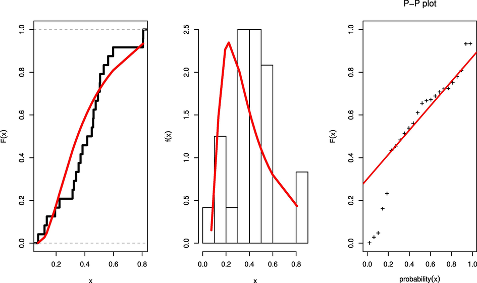
Estimated cdf, pdf and PP plot for NUL distribution.

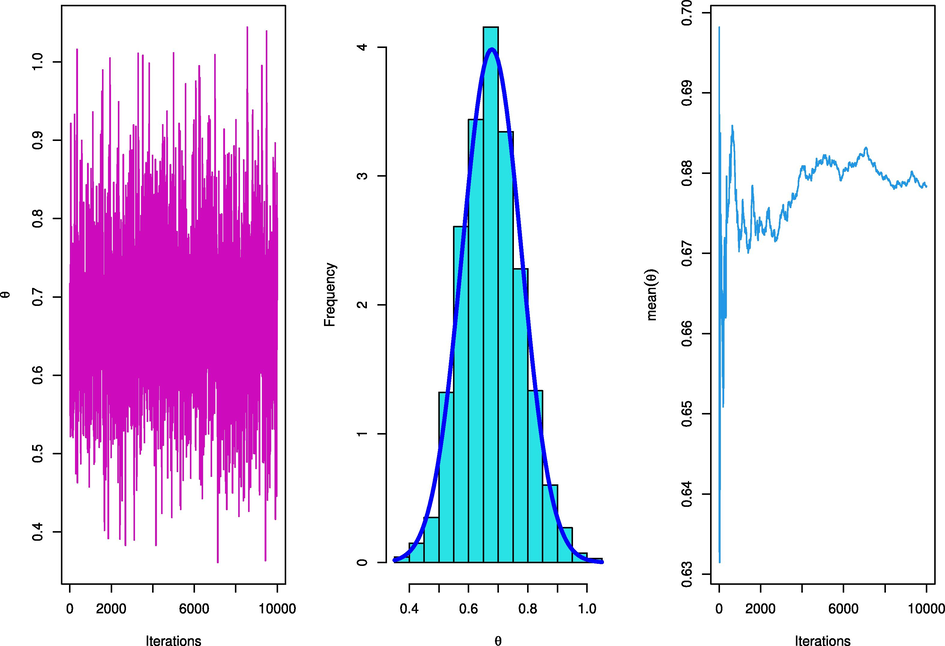
The trace plots and marginal posterior probability density function of the parameter.

7 Conclusion remarks

We evaluated the maximum likelihood and Bayes estimators of unknown parameters using an adaptive Type-II progressive hybrid censoring scheme. Additionally, we evaluated the reliability and hazard rate functions of the NUL model.The square error loss function is used to determine the Bayes estimators. We employed the M-H algorithm and Monte Carlo Markov Chain methods because the Bayes estimators aren’t available in closed form. The performance of the suggested technique is investigated Monte Carlo simulation for several points and interval technique. A real data set of repairable mechanical equipment item sets is investigated to prove applicability of the presented concept. The obtained results proved that the suggested approach in the paper is valuable to data analysts and reliability practitioners. In the future work, we can study the derivation of Bayes estimates based on truncated independent normal priors in comparison with the obtained the results in this paper.

Acknowledgment

This research received funding support from the NSRF via the Program Management Unit for Human Resources & Institutional Development, Research and Innovation, (Grant No. B05F650018).

Declaration of Competing Interest

The authors declare that they have no known competing financial interests or personal relationships that could have appeared to influence the work reported in this paper.

References

Ahmad H.H., Almetwally E.M., Ramadan D.A., . A comparative inference on reliability estimation for a multi-component stress-strength model under power Lomax distribution with applications. AIMS Math. 2022;7:18050-18079.
[Google Scholar]
Alkhairy Ibrahim, . A new flexible logarithmic-X family of distributions with applications to biological systems. Complexity. 2022;2022
[Google Scholar]
Almetwally E.M., Almongy H.M., ElSherpieny E.A., . Adaptive Type-II progressive censoring schemes based on maximum product spacing with application of generalized Rayleigh distribution. J. Data Sci.. 2019;17(4):802-831.
[Google Scholar]
Almetwally E.M., Almongy H.M., Rastogi M.K., Ibrahim M., . Maximum product spacing estimation of Weibull distribution under adaptive type-II progressive censoring schemes. Ann. Data Sci.. 2020;7(2):257-279.
[Google Scholar]
Almetwally E.M., Jawa T.M., Sayed-Ahmed N., Park C., Zakarya M., Dey S., . Analysis of unit-Weibull based on progressive type-II censored with optimal scheme. Alexandria Eng. J.. 2023;63(1):321-338.
[CrossRef] [Google Scholar]
Alshenawy R., Al-Alwan A., Almetwally E.M., Afify A.Z., Almongy H.M., . Progressive type-II censoring schemes of extended odd Weibull exponential distribution with applications in medicine and engineering. Mathematics. 2020;8(10):1679.
[Google Scholar]
Alshenawy R., Sabry M.A., Almetwally E.M., Almongy H.M., . Product spacing of stress–strength under progressive hybrid censored for exponentiated-gumbel distribution. Comput. Mater. Continua. 2021;66(3):2973-2995.
[Google Scholar]
Alsuhabi Hassan, . A superior extension for the Lomax distribution with application to Covid-19 infections real data. Alexandria Eng. J.. 2022;61(12):11077-11090.
[Google Scholar]
Alyami S.A., Elbatal I., Alotaibi N., Almetwally E.M., Elgarhy M., . Modeling to factor productivity of the United Kingdom Food Chain: using a new lifetime-generated family of distributions. Sustainability. 2022;14(14):8942.
[Google Scholar]
Anatolyev S., Kosenok G., . An alternative to maximum likelihood based on spacings. Econometric Theory. 2005;21(2):472-476.
[Google Scholar]
Aslam M., Huang S.R., Chi H.J., Ahmad M., Rasool M., . A reliability sampling plan based on progressive interval censoring under Pareto distribution of second kind. Ind. Eng. Manage. Syst.. 2011;10(2):154-160.
[Google Scholar]
Aslam M., Arif O.H., Jun C.H., . An attribute control chart for a Weibull distribution under accelerated hybrid censoring. PloS One. 2017;12(3):e0173406.
[Google Scholar]
Aslam, M., Rao, G.S., Saleem, M., Sherwani, R.A.K., Jun, C.H., 2021. Monitoring mortality caused by COVID-19 using gamma-distributed variables based on generalized multiple dependent state sampling. Comput. Mathe. Methods Med. 2021.
Balakrishnan N., Aggarwala R., . Progressive Censoring Theory, Methods and Applications. Boston, MA: Birkhäuser; 2000.
Balakrishnan N., Cramer E., . The Art of Progressive Censoring. Birkhäuser, New York: Springer; 2014.
Biswas A., Chakraborty S., . Stress-strength reliability for the unit-lindley distribution with an application. Calcutta Stat. Assoc. Bull.. 2021;73(1):7-23.
[Google Scholar]
Chen M.H., Shao Q.M., . Monte Carlo estimation of Bayesian credible and HPD intervals. J. Comput. Graphical Stat.. 1999;8:69-92.
[Google Scholar]
Cheng R.C.H., Amin N.A.K., . Estimating parameters in continuous univariate distributions with a shifted origin. J. Roy. Stat. Soc. B. 1983;45(3):394-403.
[Google Scholar]
El-Sherpieny E.S.A., Almetwally E.M., Muhammed H.Z., . Progressive Type-II hybrid censored schemes based on maximum product spacing with application to Power Lomax distribution. Physica A. 2020;553:124251.
[Google Scholar]
Gelman A., Carlin J.B., Stern H.S., Rubin D.B., . Bayesian Data Analysis (2nd ed.). USA: Chapman and Hall/CRC; 2004.
Goel R., Krishna H., . Progressive type-II random censoring scheme with Lindley failure and censoring time distributions. Int. J. Agric. Stat. Sci.. 2020;16(1):23-34.
[Google Scholar]
Greene W.H., . Econometric Analysis (4th ed.). NewYork: Prentice-Hall; 2000.
Hafez E.H., Riad F.H., Mubarak S.A., Mohamed M.S., . Study on Lindley distribution accelerated life tests: Application and numerical simulation. Symmetry. 2020;12(12):2080.
[Google Scholar]
Irshad M.R., D’cruz V., Maya R., . The exponentiated unit Lindley distribution: properties and applications. Ricerche mat.. 2021;1–23
[CrossRef] [Google Scholar]
Lawless J.F., . Statistical Models and Methods For Lifetime Data (2nd ed.). New Jersey: John Wiley and Sons; 2003.
Lin Yushan, . Impact of facebook and newspaper advertising on sales: a comparative study of online and print media. Comput. Intell. Neurosci. 2021 (2021).
[Google Scholar]
Lynch S.M., . Introduction to Applied Bayesian Statistics and Estimation for Social Scientists. New York: Springer; 2007.
Mazucheli J., Menezes A.F.B., Chakraborty S., . On the one parameter unit-Lindley distribution and its associated regression model for proportion data. J. Appl. Stat.. 2019;46(4):700-714.
[Google Scholar]
Mazucheli J., Bapat S.R., Menezes A.F.B., . A new one-parameter unit-Lindley distribution. Chilean J. Stat. (ChJS). 2020;11(1):53-67.
[Google Scholar]
Nadarajah S., Chan S., . On moments of the unit Lindley distribution. J. Appl. Stat.. 2020;47(5):947-949.
[Google Scholar]
Ng H.K.T., Chan P.S., Balakrishnan N., . Optimal progressive censoring plans for the Weibull distribution. Technometrics. 2004;46:470-481.
[Google Scholar]
Ng H.K.T., Kundu D., Chan P.S., . Statistical analysis of exponential lifetimes under an adaptive Type-II progressive censoring scheme. Naval Res. Logist.. 2009;56(8):687-698.
[Google Scholar]
Pradhan B., Kundu D., . Inference and optimal censoring schemes for progressively censored Birnbaum-Saunders distribution. J. Stat. Plann. Inference. 2013;143:1098-1108.
[Google Scholar]
Ranneby B., . The maximum spacing method. An estimation method related to the maximum likelihood method. Scand. J. Stat.. 1984;11:93-112.
[Google Scholar]
Rao G.S., Aslam M., . Inspection plan for COVID-19 patients for Weibull distribution using repetitive sampling under indeterminacy. BMC Med. Res. Methodol.. 2021;21(1):1-15.
[Google Scholar]
Sherwani R.A.K., Shakeel H., Saleem M., Awan W.B., Aslam M., Farooq M., . A new neutrosophic sign test: An application to COVID-19 data. PloS One. 2021;16(8):e0255671.
[Google Scholar]
Wang Yongjing, . Analysis of cryptocurrency exchange rates vs USA dollars using a new Dagum model. Alexandria Eng. J. 2022
[Google Scholar]
Zhou Yang, . Impact of YouTube Advertising on Sales with Regression Analysis and Statistical Modeling: Usefulness of Online Media in Business. Comput. Intell. Neurosci.. 2021;2021
[Google Scholar]

Show Sections

[1] Ahmad H.H., Almetwally E.M., Ramadan D.A., . A comparative inference on reliability estimation for a multi-component stress-strength model under power Lomax distribution with applications. AIMS Math. 2022;7:18050-18079.
[Google Scholar]

[2] Alkhairy Ibrahim, . A new flexible logarithmic-X family of distributions with applications to biological systems. Complexity. 2022;2022
[Google Scholar]

[3] Almetwally E.M., Almongy H.M., ElSherpieny E.A., . Adaptive Type-II progressive censoring schemes based on maximum product spacing with application of generalized Rayleigh distribution. J. Data Sci.. 2019;17(4):802-831.
[Google Scholar]

[4] Almetwally E.M., Almongy H.M., Rastogi M.K., Ibrahim M., . Maximum product spacing estimation of Weibull distribution under adaptive type-II progressive censoring schemes. Ann. Data Sci.. 2020;7(2):257-279.
[Google Scholar]

[5] Almetwally E.M., Jawa T.M., Sayed-Ahmed N., Park C., Zakarya M., Dey S., . Analysis of unit-Weibull based on progressive type-II censored with optimal scheme. Alexandria Eng. J.. 2023;63(1):321-338.
[CrossRef] [Google Scholar]

[6] Alshenawy R., Al-Alwan A., Almetwally E.M., Afify A.Z., Almongy H.M., . Progressive type-II censoring schemes of extended odd Weibull exponential distribution with applications in medicine and engineering. Mathematics. 2020;8(10):1679.
[Google Scholar]

[7] Alshenawy R., Sabry M.A., Almetwally E.M., Almongy H.M., . Product spacing of stress–strength under progressive hybrid censored for exponentiated-gumbel distribution. Comput. Mater. Continua. 2021;66(3):2973-2995.
[Google Scholar]

[8] Alsuhabi Hassan, . A superior extension for the Lomax distribution with application to Covid-19 infections real data. Alexandria Eng. J.. 2022;61(12):11077-11090.
[Google Scholar]

[9] Alyami S.A., Elbatal I., Alotaibi N., Almetwally E.M., Elgarhy M., . Modeling to factor productivity of the United Kingdom Food Chain: using a new lifetime-generated family of distributions. Sustainability. 2022;14(14):8942.
[Google Scholar]

[10] Anatolyev S., Kosenok G., . An alternative to maximum likelihood based on spacings. Econometric Theory. 2005;21(2):472-476.
[Google Scholar]

[11] Aslam M., Huang S.R., Chi H.J., Ahmad M., Rasool M., . A reliability sampling plan based on progressive interval censoring under Pareto distribution of second kind. Ind. Eng. Manage. Syst.. 2011;10(2):154-160.
[Google Scholar]

[12] Aslam M., Arif O.H., Jun C.H., . An attribute control chart for a Weibull distribution under accelerated hybrid censoring. PloS One. 2017;12(3):e0173406.
[Google Scholar]

[13] Aslam, M., Rao, G.S., Saleem, M., Sherwani, R.A.K., Jun, C.H., 2021. Monitoring mortality caused by COVID-19 using gamma-distributed variables based on generalized multiple dependent state sampling. Comput. Mathe. Methods Med. 2021.

[14] Balakrishnan N., Aggarwala R., . Progressive Censoring Theory, Methods and Applications. Boston, MA: Birkhäuser; 2000.

[15] Balakrishnan N., Cramer E., . The Art of Progressive Censoring. Birkhäuser, New York: Springer; 2014.

[16] Biswas A., Chakraborty S., . Stress-strength reliability for the unit-lindley distribution with an application. Calcutta Stat. Assoc. Bull.. 2021;73(1):7-23.
[Google Scholar]

[17] Chen M.H., Shao Q.M., . Monte Carlo estimation of Bayesian credible and HPD intervals. J. Comput. Graphical Stat.. 1999;8:69-92.
[Google Scholar]

[18] Cheng R.C.H., Amin N.A.K., . Estimating parameters in continuous univariate distributions with a shifted origin. J. Roy. Stat. Soc. B. 1983;45(3):394-403.
[Google Scholar]

[19] El-Sherpieny E.S.A., Almetwally E.M., Muhammed H.Z., . Progressive Type-II hybrid censored schemes based on maximum product spacing with application to Power Lomax distribution. Physica A. 2020;553:124251.
[Google Scholar]

[20] Gelman A., Carlin J.B., Stern H.S., Rubin D.B., . Bayesian Data Analysis (2nd ed.). USA: Chapman and Hall/CRC; 2004.

[21] Goel R., Krishna H., . Progressive type-II random censoring scheme with Lindley failure and censoring time distributions. Int. J. Agric. Stat. Sci.. 2020;16(1):23-34.
[Google Scholar]

[22] Greene W.H., . Econometric Analysis (4th ed.). NewYork: Prentice-Hall; 2000.

[23] Hafez E.H., Riad F.H., Mubarak S.A., Mohamed M.S., . Study on Lindley distribution accelerated life tests: Application and numerical simulation. Symmetry. 2020;12(12):2080.
[Google Scholar]

[24] Irshad M.R., D’cruz V., Maya R., . The exponentiated unit Lindley distribution: properties and applications. Ricerche mat.. 2021;1–23
[CrossRef] [Google Scholar]

[25] Lawless J.F., . Statistical Models and Methods For Lifetime Data (2nd ed.). New Jersey: John Wiley and Sons; 2003.

[26] Lin Yushan, . Impact of facebook and newspaper advertising on sales: a comparative study of online and print media. Comput. Intell. Neurosci. 2021 (2021).
[Google Scholar]

[27] Lynch S.M., . Introduction to Applied Bayesian Statistics and Estimation for Social Scientists. New York: Springer; 2007.

[28] Mazucheli J., Menezes A.F.B., Chakraborty S., . On the one parameter unit-Lindley distribution and its associated regression model for proportion data. J. Appl. Stat.. 2019;46(4):700-714.
[Google Scholar]

[29] Mazucheli J., Bapat S.R., Menezes A.F.B., . A new one-parameter unit-Lindley distribution. Chilean J. Stat. (ChJS). 2020;11(1):53-67.
[Google Scholar]

[30] Nadarajah S., Chan S., . On moments of the unit Lindley distribution. J. Appl. Stat.. 2020;47(5):947-949.
[Google Scholar]

[31] Ng H.K.T., Chan P.S., Balakrishnan N., . Optimal progressive censoring plans for the Weibull distribution. Technometrics. 2004;46:470-481.
[Google Scholar]

[32] Ng H.K.T., Kundu D., Chan P.S., . Statistical analysis of exponential lifetimes under an adaptive Type-II progressive censoring scheme. Naval Res. Logist.. 2009;56(8):687-698.
[Google Scholar]

[33] Pradhan B., Kundu D., . Inference and optimal censoring schemes for progressively censored Birnbaum-Saunders distribution. J. Stat. Plann. Inference. 2013;143:1098-1108.
[Google Scholar]

[34] Ranneby B., . The maximum spacing method. An estimation method related to the maximum likelihood method. Scand. J. Stat.. 1984;11:93-112.
[Google Scholar]

[35] Rao G.S., Aslam M., . Inspection plan for COVID-19 patients for Weibull distribution using repetitive sampling under indeterminacy. BMC Med. Res. Methodol.. 2021;21(1):1-15.
[Google Scholar]

[36] Sherwani R.A.K., Shakeel H., Saleem M., Awan W.B., Aslam M., Farooq M., . A new neutrosophic sign test: An application to COVID-19 data. PloS One. 2021;16(8):e0255671.
[Google Scholar]

[37] Wang Yongjing, . Analysis of cryptocurrency exchange rates vs USA dollars using a new Dagum model. Alexandria Eng. J. 2022
[Google Scholar]

[38] Zhou Yang, . Impact of YouTube Advertising on Sales with Regression Analysis and Statistical Modeling: Usefulness of Online Media in Business. Comput. Intell. Neurosci.. 2021;2021
[Google Scholar]

Optimal analysis of adaptive type-II progressive censored for new unit-lindley model

Abstract

Keywords

Adaptive Type-II progressive censoring

Bayesian estimator

Bootstrapping

Metropolis-Hasting algorithm

Reliability

Unit-Lindley distribution

1 Introduction

2 Classical inference

2.1 Maximum likelihood estimator

2.2 Maximum product of spacings estimators

2.3 Asymptotic confidence intervals

3 Bayesian estimators

3.1 Prior information and loss function

3.2 Posterior analysis by LF

4 Optimum progressive censoring plans

5 Generating simulated data data for estimation purpose

5.1 Simulation purpose

5.2 Simulation design

5.3 Simulation outcome observations

6 Real-life applications

7 Conclusion remarks

Acknowledgment

Declaration of Competing Interest

References

Suggested read for related articles: