

Translate this page into:
On the soliton solutions to the modified Benjamin-Bona-Mahony and coupled Drinfel’d-Sokolov-Wilson models and its applications
⁎Corresponding author at: Mathematics Department, Faculty of Science, Taibah University, Al-Madinah Al-Munawarah, Saudi Arabia. aly742001@yahoo.com (Aly R. Seadawy) aabdelalim@taibahu.edu.sa (Aly R. Seadawy)
-
Received: ,
Accepted: ,
This article was originally published by Elsevier and was migrated to Scientific Scholar after the change of Publisher.
Peer review under responsibility of King Saud University.
Abstract
In this article, the analytical solutions for modified Benjamin-Bona-Mahony and coupled Drinfel’d-Sokolov-Wilson equations have been extracted with the help of very simple transformation. These results hold numerous traveling wave solutions that are of key importance in elucidating some physical circumstance. The technique can also be functional to other sorts of nonlinear evolution equations in contemporary areas of research.
Keywords
Modified Benjamin-Bona-Mahony equation
Drinfel’d-Sokolov-Wilson equation
Auxiliary equation method

1 Introduction
Nonlinear evolution equations (NEEs) have been studied in last few decades. A verity of NEEs are integrated with the help of various interesting computational techniques. To understand the physical structure, described by nonlinear partial differential equations (PDEs), exact solutions to the nonlinear PDEs play a crucial role in the study of the nonlinear models appearing in diverse disciplines; for instance, electromagnetic theory, geochemistry, astrophysics, fluid dynamics, elastic media, nuclear physics, optical fibers, high-energy physics, gravitation and in statistical and condensed matter physics, biology, solid state physics, chemical kinematics, chemical physics, electrochemistry, fluid dynamics, acoustics, cosmology and plasma physics etc, see (Seadawy and El-Rashidy, 2013; Gardner et al., 1967; Su and Gardner, 1969; Ito, 1980; Zhibin and Mingliang, 1993; Liang, 2014; Seadawy, 2012a,b; Seadawy, 2016a,b).
In recent few decades, growing interest have been drawn to find the analytical solutions for nonlinear wave equations, such as the traveling wave solution (Xu and Li, 2005), Cole-Hopf transformation, Painlevé method, Bäcklund transformation, amplitude ansatz method (Seadawy and Lu, 2017), sine-cosine method, Darboux transformation, Hirota method, function transformation method, Lie group analysis, extended simple equation method (Lu et al., 2017), homogeneous balance method (Chen et al., 2003), similarity reduced method, tanh method, fractional direct algebraic function method (Seadawy, 2016), inverse scattering method (Ablowitz and Clarkson, 1991), Hirota’s bilinear method (Hirota, 1971), the homogeneous balance method (Wang, 1995), variational method (Khater et al., 2003), algebraic method (Khater et al., 2000), sine-cosine method, Jacobi elliptic function method (Liu et al., 2001), the F-expansion method (Zhou et al., 2003), extended Fan Sub-Equation method (Kalim and Younis, 2017), the expansion method (Abazari, 2010; Kutluay et al., 2010), the tanh and extended tanh method, extended direct algebraic method (Seadawy et al., 2016), the auxiliary equation method (Kalim and Seadawy, 2017) and many more (Yan et al., 2012; Grey and Tom, 2014; Mohapatra et al., 2015; Kalim and Seadawy, 2019; Abu Arqub et al., 2015; El-Ajou et al., 2015a,b; Abu Arqub, 2017a,b).
In this paper, the auxiliary equation method (AEM) is applied to construct the traveling wave solutions to the modified Benjamin-Bona-Mahony (m-BBM) and coupled Drinfel’d-Sokolov-Wilson (c-DSW) equations. The aim of the study is to deal with the explicit solutions of NPDEs and to explore the configuration of the physical phenomena depending upon various parameters. As a result, some new and more general exact traveling wave solutions are obtained.
The Benjamin-Bona-Mahony equation (BBM) describes the unidirectional propagation of long waves in certain nonlinear dispersive media, as discussed in Seadawy (2018, 2017). The BBM equation is known as the modified BBM equation (mBBM) for
. The governing equation is as follows:
The coupled Drinfel’d-Sokolov-Wilson system (cDSW) reads
This article has been devised as follows: in Section 2, the auxiliary equation method is introduced, while in Section 3, the solutions of the NPDEs have been presented. In last Section 4, the conclusions have been drawn.
2 The description of the auxiliary equation method
We will briefly present the AEM in the following steps:
-
Step 1.
Let us have a general form of nonlinear PDE
(3)where F is a polynomial function with respect to the indicated variables. -
Step 2.
-
Step 3.
The main idea of the auxiliary equation method based on expanding the traveling wave solution of Eqs. (5) as a finite series
(6)satisfies
(7)(8)where and are constants. -
Step 4.
-
Step 5.
-
Step 6.
3 Soliton extraction
3.1 Modified Benjamin-Bona-Mahony equation
Consider the transformation
Case I.
(a).
(13)
,
,
,
,
,
, where
and
are arbitrary constants, hence the solution of (1) will be
(b).
(15)
,
,
,
,
,
, where
and
are arbitrary constants, hence the solution of (1) will be
Case II.
(a).
(18)
,
,
,
,
,
,
, where
and
are arbitrary constants, hence the solution of (1) will be
(b).
(21)
,
,
,
,
,
,
where
and
are arbitrary constants, hence the solution of (1) will be
(c).
(24)
,
,
,
,
,
,
where
is arbitrary constant, hence the solution of (1) will be
Case III.
(a).
(27)
,
,
,
,
,
,
, where
is arbitrary constant, hence the solution of (1) will be
(b).
(30)
,
,
,
,
,
, where
is arbitrary constant, hence the solution of (1) will be
3.2 Coupled Drinfel’d-Sokolov-Wilson equation
Consider the transformation
Case I.
(a).
(39)
,
,
,
,
,
,
, where
is arbitrary constant, hence the solution of (2) will be
(b).
(41)
,
,
,
,
,
,
, where
is arbitrary constant, hence the solution of (2) will be
Case II.
(a).
(43)
,
,
,
,
,
,
, where
is arbitrary constant, hence the solution of (1) will be
(b).
(46)
,
,
,
,
,
where
is arbitrary constant, hence the solution of (1) will be
Case III.
(a).
(49)
,
,
,
,
,
where
is arbitrary constant, hence the solution of (2) will be
(b).
(52)
,
,
,
,
,
where
and
are arbitrary constants, hence the solution of (2) will be
4 Discussions and results
The graphical representation of solitons have been illustrated in the following figures, for various values of the parameters. Mathematica 10.4 is used to carried out simulations and to visualize the behavior of nonlinear waves. In Case I, the solution for the Eq. (1), is shown in Fig. 1 obtained from the Eq. (14) with
,
,
,
, and Eq. (17) with
,
,
,
, while in Case II, the solution for the Eq. (1), is shown in Fig. 2 obtained from the Eq. (20) with
,
,
,
, Eq. (23) with
,
,
,
and Eq. (26) with
,
,
,
. Moreover, in Case III, the solution for the Eq. (1), is shown in Fig. 3 obtained from the Eq. (29) with
,
,
,
,
and Eq. (32) with
,
,
,
,
.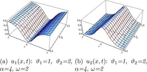
mBBM equation (Case I).
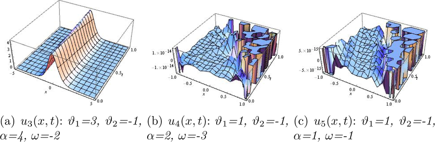
mBBM equation (Case II).
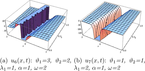
mBBM equation (Case III).
Similarly, the solution to the Eq. (2) for Case I, is shown in Fig. 4 obtained from the Eq. (40) with
,
,
,
,
,
and Eq. (42) with
,
,
,
,
,
, while In Case II, the solution for the Eq. (2), is shown in Fig. 5 obtained from the Eqs. (45) with
,
,
,
,
,
,
and Eq. (48) with
,
,
,
,
,
,
. Moreover, in Case III, the solution for the Eq. (2), is shown in Fig. 6 obtained from the Eq. (51) with
,
,
,
,
,
,
and Eq. (53) with
,
,
,
,
,
.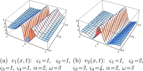
cDSW system (Case I).
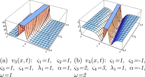
cDSW system (Case II).
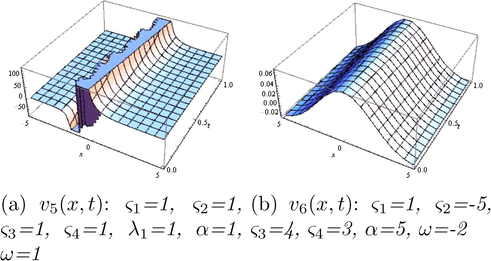
cDSW system (Case III).
5 Conclusion
The aim of the study is to find some new traveling-wave solutions for modified Benjamin-Bona-Mahony and Drinfel’d-Sokolov-Wilson equations. It is observed that the auxiliary equation method is one of the most powerful tools to find a variety of analytical solutions for more complex problems. Depending on the real parameters, a collection of new exact solutions are obtained, for details see Figs. 1–6 These results are very auspicious for further investigation and stances on a strong basis for the solution of NPDEs.
References
- Application of -expansion method to travelling wave solutions of three nonlinear evolution equation. Comput. Fluids. 2010;39:1957-1963.
- [Google Scholar]
- Soliton, Nonlinear Evolution Equations and Inverse Scattering. Cambridge University Press, USA; 1991.
- Numerical solutions for the Robin time-fractional partial differential equations of heat and fluid flows based on the reproducing kernel algorithm. Int. J. Numer. Meth. Heat Fluid Flow 2017
- [CrossRef] [Google Scholar]
- Fitted reproducing kernel Hilbert space method for the solutions of some certain classes of time-fractional partial differential equations subject to initial and Neumann boundary conditions. Comput. Math. Appl.. 2017;73:1243-1261.
- [Google Scholar]
- Constructing and predicting solitary pattern solutions for nonlinear time-fractional dispersive partial differential equations. J. Comput. Phys.. 2015;293:385-399.
- [Google Scholar]
- New explicit solitary wave solutions for (2 + 1)-dimensional Boussinesq equation and (3 + 1)-dimensional KP equation. Phys. Lett. A. 2003;307:107-113.
- [Google Scholar]
- A novel expansion iterative method for solving linear partial differential equations of fractional order. Appl. Math. Comput.. 2015;257:119-133.
- [Google Scholar]
- Approximate analytical solution of the nonlinear fractional KdV-Burgers equation: a new iterative algorithm. J. Comput. Phys.. 2015;293:81-95.
- [Google Scholar]
- Method for solving the Korteweg-de Vries equation. Phys. Rev. Lett.. 1967;19:1095-1097.
- [Google Scholar]
- Grey Jacob, Michael M. Tom, 2014. On the Solutions of the BBM-KP and BBM model Equations, oai:arXiv.org: 1410.3158.
- Exact solution of the Korteweg-de Vries equation for multiple collisions of solitons. Phys. Rev. Lett.. 1971;27:1192-1194.
- [Google Scholar]
- An extension of nonlinear evolution equation of the K-dV(mKdV) type to higher order. J. Phys. Soc. Jpn.. 1980;49:771-778.
- [Google Scholar]
- Bistable Bright-Dark Solitary Wave Solutions of the (3 + 1)-Dimensional Breaking Soliton, Boussinesq Equation with Dual Dispersion and Modified KdV-KP equations and their applications. Results Phys.. 2017;7:1143-1149.
- [Google Scholar]
- Soliton Solution of (3 + 1)-Dimensional KdV-BBM, KP-BBM and mKdV-ZK equations and their applications in water waves. J. King Saud Univ.- Sci.. 2019;31:8-13.
- [Google Scholar]
- Bright, dark and other optical solitons with second order spaotetimporal dispersion. Optik. 2017;142:446-450.
- [Google Scholar]
- General soliton solutions of an n-dimensional Complex Ginzburg-Landau equation. Phys. Scr.. 2000;62:353-357.
- [Google Scholar]
- Khater, A.H., Callebaut D.K., Seadawy A.R., 2003. Nonlinear Dispersive Kelvin-Helmholtz Instabilities in Magnetohydrodynamic Flows Presented in International Conference on Computational and Applied Mathematics (Belgium) ICCAM 2000 and published in Physica Scripta, 67, 340–349.
- Variational method for the nonlinear dynamics of an elliptic magnetic stagnation line. Eur. Phys. J. D. 2006;39:237-245.
- [Google Scholar]
- The -expansion method for some nonlinear evolution equations. Appl. Math. Comput.. 2010;217:384-391.
- [Google Scholar]
- Exact solutions of the (3 + 1)-dimensional modified KdV-Zakharov-Kuznetsev equation and Fisher equations using the modified simple equation method. J. Interdisciplinary Math.. 2014;17:565-578.
- [Google Scholar]
- Jacobi elliptic function expansion method and periodic wave solutions of nonlinear wave equations. Phys. Lett. A. 2001;289:69-74.
- [Google Scholar]
- Applications of extended simple equation method on unstable nonlinear Schrödinger equations. Optik. 2017;140:136-144.
- [Google Scholar]
- Mohapatra, S.C., Guedes Soares, C., 2015. Comparing solutions of the coupled Boussinesq equations in shallow water. In: Guedes Soares, Santos (Eds.), Maritime Technology and Engineering. Taylor & Francis Group, London, ISBN 978-1-138-02727-5.
- Exact solutions of a two-dimensional nonlinear Schrödinger equation. Appl. Math. Lett.. 2012;25:687-691.
- [Google Scholar]
- Traveling wave solutions of the Boussinesq and generalized fifth-order KdV equations by using the direct algebraic method. Appl. Math. Sci.. 2012;6(82):4081-4090.
- [Google Scholar]
- Three-dimensional nonlinear modified Zakharov-Kuznetsov equation of ion-acoustic waves in a magnetized plasma. Comput. Math. Appl.. 2016;71:201-212.
- [Google Scholar]
- Stability analysis solutions for nonlinear three-dimensional modified Korteweg-de Vries-Zakharov-Kuznetsov equation in a magnetized electron-positron plasma. Physica A. 2016;455:44-51.
- [Google Scholar]
- Stability analysis of traveling wave solutions for generalized coupled nonlinear KdV equations. Appl. Math. Inf. Sci.. 2016;10:209-214.
- [Google Scholar]
- Solitary wave solutions of tow-dimensional nonlinear Kadomtsev-Petviashvili dynamic equation in a dust acoustic plasmas. The Pramana – J. Phys.. 2017;89(3) 49:1–11
- [Google Scholar]
- Two-dimensional interaction of a shear flow with a free surface in a stratified fluid and its a solitary wave solutions via mathematical methods. Eur. Phys. J. Plus. 2017;132 518:12, 1–11
- [Google Scholar]
- Three-dimensional weakly nonlinear shallow water waves regime and its travelling wave solutions. Int. J. Comput. Methods. 2018;15(1)
- [Google Scholar]
- Mathematical methods via the nonlinear two-dimensional water waves of Olver dynamical equation and its exact solitary wave solutions. Results Phys.. 2018;8:286-291.
- [Google Scholar]
- Traveling wave solutions for some coupled nonlinear evolution equations. Math. Comput. Model.. 2013;57:1371-1379.
- [Google Scholar]
- Bright and dark solitary wave soliton solutions for the generalized higher order nonlinear Schrödinger equation and its stability. Results Phys.. 2017;7:43-48.
- [Google Scholar]
- Water wave solutions of Zufiria?s higher-order Boussinesq type equations and its stability. Appl. Math. Comput.. 2016;280:57-71.
- [Google Scholar]
- Drivation of the Korteweg-de Vries and Burgers Equation. J. Math. Phys.. 1969;10:536-539.
- [Google Scholar]
- Solitary wave solutions for variant Boussinesq equations. Phys. Lett. A. 1995;199:169-172.
- [Google Scholar]
- New exact solutions for the classical Drinfel’d-Sokolov-Wilson equation. Appl. Math. Comput.. 2009;215:2349-2358.
- [Google Scholar]
- Exact travelling wave solutions of the Whitham-Broer-Kaup and Broer-Kaup-Kupershmidt equations. Chaos, Solitons Fractals. 2005;24:549-556.
- [Google Scholar]
- The exact traveling wave solutions and their bifurcations in the Gardner and Gardner-KP Equations. Int. J. Bifurcation Chaos. 2012;22(5):125-126.
- [Google Scholar]
- Travelling wave solutions to the two-dimensional Kdv-Burgers equation. J. Phys. A: Math. Gen.. 1993;26:6027-6031.
- [Google Scholar]
- Periodic wave solutions to a coupled KdV equations with variable coefficients. Phys. Lett. A. 2003;308:31-36.
- [Google Scholar]


