On the comparative study integro – Differential equations using difference numerical methods

Shams A. Ahmed; Tarig M. Elzaki

doi:10.1016/j.jksus.2018.03.003

View/Download PDF

Buy Reprints

PDF

Translate this page into:

Original article

32 (

); 84-89

doi:

10.1016/j.jksus.2018.03.003

On the comparative study integro – Differential equations using difference numerical methods

Shams A. Ahmed^{^a,^b}, Tarig M. Elzaki^{^c,⁎}

a Department of Mathematic, Faculty of Sciences and Arts-Tubarjal, Aljouf University, Saudi Arabia

b Department of Mathematic, University of Gezira, Sudan

c Mathematics Department, Faculty of Sciences and Arts, Alkamil, Jeddah, University of Jeddah, Saudi Arabia

⁎Corresponding author. tarig.alzaki@gmail.com (Tarig M. Elzaki)

Received: 2018-1-12, Accepted: 2018-3-7, Published: 2018-01-01

Disclaimer:
This article was originally published by Elsevier and was migrated to Scientific Scholar after the change of Publisher.

Peer review under responsibility of King Saud University.

Abstract

In this paper, we use the Adomian decomposition Sumudu transform method with the Pade approximant (ADST - PA method) to obtain closed form solutions of nonlinear integro-differential equations, and perform a comparative study between the present method and three different numerical methods, namely; the Adomian decomposition Sumudu transform method (ADSTM)), the homotopy perturbation method (HPM), and the variational iteration method (VIM). Our results show that in comparison with other existing methods, the (ADST - PA method) gives a better approximation for solving a large number of nonlinear integro-differential equations than existing methods.

Keywords

Adomian decomposition Sumudu transform method

Homotopy perturbation method

Pade approximant

Variational iteration method

Integro-differential equation

Show Related Articles from PubMed

1 Introduction

Ever since long time, integro differential equations have played an important part in all facets of science applications such as ice- shaping operation, heat transformer, neutron diffusion, and biological species coexisting together with increasing and falling rates of generating and diffusion process in general. In addition, it also can be found in applied mathematics, physics, and engineering applications, as well as this in models dealing with advanced integral equations such as (Golberg, 1979; Jerri, 1971; Kanwal, 1971; Miller, 1967 ).

The homotopy perturbation method (HPM) was a consequence of some pioneering ideas beginning in 1999 by His (He, 1999). Since then it has evolved into a fully -fledged theory, which was the contribution from many researchers. The HPM method was found to be an uncomplicated and accurate method to resolve a great number of nonlinear problems.

Many sources for different cases have obtained some exact and numerical solutions of the integro-differential equation (see Avudainayagam and Vani, 2000; Bahugna et al., 2009; Abu Arqub and Al-samdi, 2013; Abu Arqub and Al-samdi, 2014; Momani et al., 2014; El-ajou et al., 2012; Eltayeb et al., 2014; Ahmed and Elzaki, 2013 ).

In the present study, we consider the nonlinear integro- differential equation of the following type:

(1)

V^{'} (x) = f (x) + \int_{0}^{x} K (t, v (t), v^{'} (t)) dt,

with the initial condition;

(2)

v (0) = α, 0 ⩽ x ⩽ 1;

where

f (x)

is known as the source term and

K (t, v (t), v^{'} (t))

is a linear or nonlinear function depending on the problem discussed.

The main objective of this paper is to introduce a comparative study to solve integro-differential equation (1) by using four of the most recently developed methods, namely, the Adomian decomposition Sumudu transform method (ADSTM), the homotopy perturbation method (HPM), the variational iteration method (VIM) and the Adomian decomposition Sumudu transform method with Pade approximant (ADSTM-PA).

This paper is orderly as follows. in Section 2, we show all the numerical methods in short. Two numerical experiences are introduced in Section 3 for demonstrating the complete research. Concluding remarks are given in the last section.

2 Analysis of numerical methods

2.1

2.1 The Adomian decomposition Sumudu transform method (ADSTM)

In this section, Adomian decomposition Sumudu transform method (Kumar et al., 2012) is applied to the following classes of non-linear integro-differential equation (1).

The method depends of first applying the Sumudu transformation to both sides of Eq. (1);

(3)

S [v^{'} (x)] = S [f (x)] + S [\int_{0}^{x} K (t, v (t), v^{'} (t)) dt] .

Using the formulas of the Sumudu transform, we get:

(4)

u^{- 1} S [v (x)] - u^{- 1} v (0) = S [f (x)] + S [\int_{0}^{x} K (t, v (t), v^{'} (t)) dt] .

Using the initial condition (2), we have:

(5)

S [v (x)] = α + u S [f (x)] + u S [\int_{0}^{x} K (t, v (t), v^{'} (t)) dt]

If we apply the inverse operator $S^{- 1}$ to both sides of the Eq. (5), we obtain:

(6)

v (x) = α + S^{- 1} [u S [f (x)]] + S^{- 1} {u S [\int_{0}^{x} K (t, v (t), v^{'} (t)) dt]} .

In the Adomian decomposition Sumudu transform method we assume the solution as an infinite series, given as follows:

(7)

v = \sum_{n = 0}^{\infty} v_{n},

where the terms $v_{n}$ are to be recursively computed. Also, the nonlinear term $K (t, v (t), v^{'} (t))$ is decomposed as an infinite series of Adomian polynomials (see Adomian, 1990, 1984, 1986 ):

(8)

K (t, v (t), v^{'} (t)) = \sum_{n = 0}^{\infty} A_{n},

where

A_{n} = A_{n} (v_{1}, v_{2}, v_{3}, \dots, v_{n})

are determined by the following recursive relation:

(9)

A_{n} = \frac{1}{n!} {[\frac{d^{n}}{d λ^{n}} [\sum_{i = 0}^{\infty} (λ^{i} v_{i})]]}_{λ = 0} .

Using (7) and (8), we rewrite (6) as:

(10)

\sum_{n = 0}^{\infty} v_{n} (x) = α + S^{- 1} [u S [f (x)]] + S^{- 1} \{u S [\int_{0}^{x} \sum_{n = 0}^{\infty} A_{n} dt]\} .

Applying the linearity of the Sumudu transform, we have:

(11)

\sum_{n = 0}^{\infty} v_{n} (x) = α + S^{- 1} [u S [f (x)]] + S^{- 1} \{u [\int_{0}^{x} S [\sum_{n = 0}^{\infty} A_{n}] dt]\} .

Now we define the following iterative algorithm:

(12)

v_{0} = α + S^{- 1} [u S [f (x)]],

(13)

v_{1} = S^{- 1} \{u [\int_{0}^{x} S [A_{0}] dt]\} .

In general,

(14)

v_{k + 1} = S^{- 1} \{u [\int_{0}^{x} S [A_{k}] dt]\}, k ⩾ 1 .

As the result, the components $(v_{1}, v_{2}, v_{3}, \dots, v_{n})$ are identified and the series solution is thus entirely determined.

However, in many cases the exact solution in the closed form may also be obtained.

2.2

2.2 The Pade approximant

Here we will investigate the construction of the Pade approximates for the functions studied. The main advantage of the Pade approximation gives a better approximation of the function than truncating its Taylor series. The Pade approximation of a function is given by the ratio of two polynomials. The coefficients of the polynomial in both the numerator and the denominator are determined by using the coefficients in the Taylor series expansion of the function.

The Pade approximation of a function, symbolized by [m/n], is a rational function defined by;

(15)

[m / n] = \frac{a_{0} + a_{1} x + a_{2} x^{2} + . . . + a_{m} x^{m}}{1 + b_{1} x + b_{2} x^{2} + . . . + b_{n} x^{n}}

where we considered $b_{0} = 1$ , and numerator, denominator have no common factors.

In The (ADSTM-PA) we use the method of the Pade approximation as an after – treatment method to the solution obtained by the (ADSTM). This after – treatment method improves the accuracy of the proposed method.

2.3

2.3 Basic idea of the (HPM)

To explain (HPM), we consider (1) as:

(16)

L (v) = v^{'} (x) - f (x) - \int_{0}^{x} K (t, v (t), v^{'} (t)) dt = 0,

with solution

f (x)

. Now, we can define homotopy

H (v, p)

by,

(17)

H (v, 0) = F (v), H (v, 1) = L (v),

where

F (v)

is a functional operator with a solution

r_{0}

, obtained easily. Now, we choose a convex homotopy from:

(18)

H (v, p) = (1 - p) F (v) + p L (v) = 0

and continuously trace an implicitly defined curve from a starting point

H (r_{0}, 0)

to a solution function

H (f, 1)

. Here the parameter

p

is monotonically increasing from zero to unit along – with the trivial problem

F (v) = 0

is continuously deformed to the original problem

L (v) = 0

The (HPM) uses the homotopy parameter $p$ as an expending parameter to obtain (see Nayfeh, 1985),

(19)

v = r_{0} + p r_{1} + p^{2} r_{2} + p^{3} r_{3} + .

when

p \to 1

, Eq. (17), becomes the approximate solution of (16), i.e.

(20)

f = \underset{p \to 1 .}{\lim r_{0} + r_{1} + r_{2} + . . .}

Series (20) is convergent for most cases, and the rate of convergence depends on $L (v)$ .

2.4

2.4 Basic idea of the (VIM)

To clarify the basic ideas of (VIM) (Abassya et al., 2007), we consider Eq. (1) as correction functional as follows;

(21)

v_{n + 1} (x) = v_{n} (x) + \int_{0}^{x} λ (ζ) ((v_{n}^{'} (ζ) - f (ζ) - \int_{0}^{ζ} K (r, v (r), v^{'} (r)) dr)) d ζ .

where

λ

is general Lagrange multiplier which can be identified optimally via integrated by parts.we used here

λ = - 1

for first order integro- differential equation, substituting this value of the Lagrange multiplier into the functional (21), gives the iteration formula:

(22)

v_{n + 1} (x) = v_{n} (x) - \int_{0}^{x} (v_{n}^{'} (ζ) - f (ζ) - \int_{0}^{ζ} K (r, v (r), v^{'} (r)) dr) d ζ .

we can use the initial condition to select

v_{0} (x) = v (0) = α

. Using this selection into above the correction functional, gives the following successive approximations:

(23)

v_{0} (x) = v (0) = α,

(24)

v_{n + 1} (x) = v_{n} (x) - \int_{0}^{x} (v_{n}^{'} (ζ) - f (ζ) - \int_{0}^{ζ} K (r, v (r), v^{'} (r)) dr) d ζ .

Consequently, the exact solution may be obtained by using:

(25)

v (x) = \underset{n \to \infty}{\lim v_{n}} .

3 Application

In this section, we demonstrate the analysis of all the numerical methods by applying the methods to the following two integro- differential equations. A comparison of all methods is also given in the forms of graphs and tables, presented here.

Example 1: Consider the following integro- differential equation:

(26)

v^{'} (x) = - 1 + \int_{0}^{x} v^{2} (t) dt,

With the initial condition;

(27)

v (0) = 0, 0 ⩽ x ⩽ 1 .

Solution: Taking the Sumudu transform on both the sides of (26) gives:

(28)

u^{- 1} S [v (x)] - u^{- 1} v (0) = - 1 + S [\int_{0}^{x} v^{2} (t) dt] .

Using the initial condition (27) implies,

(29)

S [v (x)] = - u + u S [\int_{0}^{x} v^{2} (t) dt] .

If we apply the inverse operator $S^{- 1}$ to both sides of the Eq. (29), we obtain:

(30)

v (x) = S^{- 1} [- u] + S^{- 1} \{u S [\int_{0}^{x} v^{2} (t) dt]\} .

By the assumption (7) and (8), we rewrite (30) as,

(31)

\sum_{n = 0}^{\infty} v_{n} (x) = S^{- 1} [- u] + S^{- 1} \{u S [\int_{0}^{x} \sum_{n = 0}^{\infty} A_{n} dt]\}

where the nonlinear term

K (t, v (t), v^{'} (t)) = v^{2}

is decomposed in terms of the Adomian polynomials as suggested in (8). Few terms of the Adomian polynomials for

v^{2}

are given as follows:

\begin{matrix} A_{0} = v_{0}^{2}, \\ A_{1} = 2 v_{0} v_{1}, \\ A_{2} = 2 v_{0} v_{2} + v_{1}^{2}, \\ A_{3} = 2 v_{0} v_{3} + 2 v_{1} v_{2} \end{matrix}

And so on. Following the Adomian decomposition Sumudu transform method, we define an iterative scheme,

(32)

v_{0} = S^{- 1} [- u],

(33)

v_{k + 1} = S^{- 1} \{u [\int_{0}^{x} S [A_{k}] dt]\}, k ⩾ 0 .

Consequently, we obtain:

(34)

v_{0} = S^{- 1} [- u] = - x,

(35)

v_{1} = S^{- 1} [u S [\int_{0}^{x} A_{0} dt]] = \frac{x^{4}}{12},

(36)

v_{2} = S^{- 1} [u S [\int_{0}^{x} A_{1} dt]] = - \frac{x^{7}}{252},

(37)

v_{3} = S^{- 1} [u S [\int_{0}^{x} A_{2} dt]] = \frac{x^{10}}{6048},

(38)

v_{4} = S^{- 1} [u S [\int_{0}^{x} A_{3} dt]] = - \frac{x^{13}}{157248} .

Similarly, we can also find other components. Finally, the solution takes the following form:

(39)

v (x) = v_{0} + v_{1} + v_{2} + v_{3} + . . .,

or,

(40)

v (x) = - x + \frac{x^{4}}{12} - \frac{x^{7}}{252} + \frac{x^{10}}{6048} - \frac{x^{13}}{157248} + .

Notes on (ADSTM):

From the previous analysis, we can observe that:

(ADSTM) can obtain a series solution, not converge, which must be truncated. The truncated series solution is an inaccurate solution in that region, which will greatly restrict the application area of the method.
(ADSTM) needs some modification to overcome the Taylor series does not converge.

To overcome these disadvantages of ADSTM, the following ADSTM - PA method is suggested.

The [m/n] Pade approximant of the infinite series (40), with $m ⩾ 4$ and $n ⩾ 4$ , which gives the following rational fraction approximation to the solution:

(41)

v (x) = \frac{- x + \frac{x^{2}}{28}}{1 + \frac{x^{3}}{21}} .

Example 2: Consider the following integro- differential equation (Figs. 1 and 2):

(42)

v^{'} (x) = 1 + \int_{0}^{x} v (t) v^{'} (t) dt,

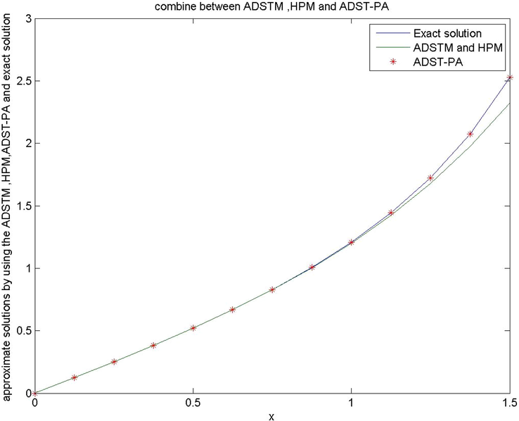
Comparison between (ADSTM), (HPM) and (ADST-PA), for Example 2.

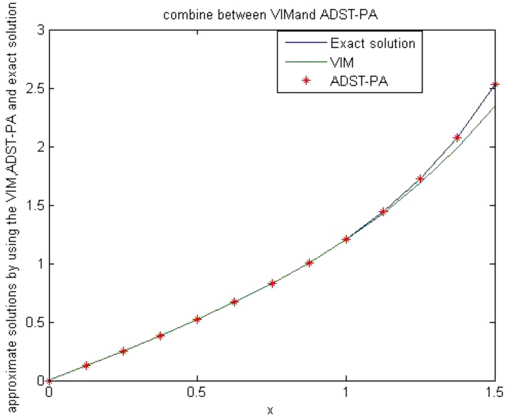
Comparison between (ADST-PA) and (VIM), for Example 2.

Given the initial condition;

(43)

v (0) = 0, 0 ⩽ x ⩽ .

With the exact solution:

(44)

v (x) = \sqrt{2} \tan (\frac{x}{\sqrt{2}}) .

Solution: Proceeding as in Example 1, Eq. (42) becomes:

(45)

\sum_{n = 0}^{\infty} v_{n} (x) = S^{- 1} [u] + S^{- 1} \{u S [\int_{0}^{x} \sum_{n = 0}^{\infty} B_{n} dt]\} .

where the nonlinear term

K (t, v (t), v^{'} (t)) = v (t) v^{'} (t)

is decomposed in terms of the Adomian polynomials as suggested in (8). We have a few terms of the Adomian polynomials of

v (t) v^{'} (t)

which are given by:

\begin{matrix} B_{0} = v_{0} v_{0_{t}}, \\ B_{1} = v_{0} v_{1_{t}} + v_{1} v_{0_{t}}, \\ B_{2} = v_{0} v_{2_{t}} + v_{1} v_{1_{t}} + v_{2} v_{0_{t}}, \\ B_{3} = v_{0} v_{3_{t}} + v_{3} v_{0_{t}} + v_{1} v_{2_{t}} + v_{2} v_{1_{t}} . \end{matrix}

And so on. Following the Adomain decomposition Sumudu transform method, we define an iterative scheme;

(46)

v_{0} = S^{- 1} [u]

(47)

v_{k + 1} = S^{- 1} \{u [\int_{0}^{x} S [B_{k}] dt]\}, k ⩾ 0 .

Now, we obtain the following components:

(48)

v_{0} = S^{- 1} [u] = x,

(49)

v_{1} = S^{- 1} [u S [\int_{0}^{x} B_{0} dt]] = \frac{x^{3}}{6}

(50)

v_{2} = S^{- 1} [u S [\int_{0}^{x} B_{1} dt]] = \frac{x^{5}}{30},

(51)

v_{3} = S^{- 1} [u S [\int_{0}^{x} B_{2} dt]] = \frac{17 x^{7}}{2520},

Similarly, we can also find other components, then the solution takes the following form;

(52)

v (x) = v_{0} + v_{1} + v_{2} + v_{3} + . . .,

(53)

v (x) = x + \frac{x^{3}}{6} + \frac{x^{5}}{30} + \frac{17 x^{7}}{2520} + . . . .

The [m/n] Pade approximant of the infinite series (53), with $m ⩾ 4$ and $n ⩾ 4$ , which gives the following rational fraction approximation to the solution:

(54)

v (x) = \frac{x - \frac{x^{3}}{21}}{1 - \frac{3 x^{2}}{14} + \frac{x^{4}}{420}} .

Numerical outcomes shown in Tables 1 and 2 and Figs. 1 and 2 illustrate the importance of (ADST - PA method) over other numerical methods.

Table 1 Comparison between (ADSTM), (HPM) and (ADST - PA method), for Example 2.

Step Size	Exact Sol.	Error(ADSTM)	Error (ADST-PA)	Error (HPM)
0.0000	0.0000	0.0000	0.0000	0.0000
0.1250	0.1253	0.0000	0.0000	0.0000
0.2500	0.2526	0.0000	0.0000	0.0000
0.3750	0.3840	0.0000	0.0000	0.0000
0.5000	0.5219	0.0001	0.0000	0.0001
0.6250	0.6691	0.0003	0.0000	0.0003
0.7500	0.8292	0.0010	0.0000	0.0010
0.8750	1.0069	0.0030	0.0000	0.0030
1.0000	1.2085	0.0081	0.0000	0.0081
1.1250	1.4431	0.0198	0.0000	0.0198
1.2500	1.7243	0.0452	0.0000	0.0452
1.3750	2.0737	0.0979	0.0000	0.0979
1.5000	2.5275	0.2051	0.0001	0.2051

Table 2 Comparison between (ADST - PA method) and (VIM), for Example 2.

Step Size	Exact Sol.	Error (ADST-PA)	Error (VIM)
0.0000	0.0000	0.0000	0.0000
0.1250	0.1253	0.0000	0.0000
0.2500	0.2526	0.0000	0.0000
0.3750	0.3840	0.0000	0.0000
0.5000	0.5219	0.0000	0.0000
0.6250	0.6691	0.0000	0.0000
0.7500	0.8292	0.0000	0.0001
0.8750	1.0069	0.0000	0.0002
1.0000	1.2085	0.0000	0.0009
1.1250	1.4431	0.0000	0.0029
1.2500	1.7243	0.0000	0.0087
1.3750	2.0737	0.0000	0.0242
1.5000	2.5275	0.0001	0.0644

4 Concluding remarks

In this report, we have examined a few recent familiar numerical methods for solving integro-differential equations. The numerical studies showed that all the methods give highly accurate solutions for given equations. The (ADSTM), the (HPM) and the (VIM) are uncomplicated and comfortable. Despite this, they are not converging to a closed form. Since the method of the (ADSTM) is based on an approximation of the solution function in this study by the truncating of approximation the solution, this kind of approximation is an inaccurate solution, which will greatly restrict the application area of the method. To get to the more dependable of these demerits, we use the Pade approximations. This fact is indicated in the second example.

References

Abassya T.A., El-Tawil M.A., El-Zoheiry H., . Exact solutions of some nonlinear partial differential equations using the variational iteration method linked with Laplace transforms and the Pade technique. Comput. Math. Appl.. 2007;54:940-954.
[Google Scholar]
Abu Arqub O., Al-samdi M., . Solving Fredholm integro-differential equations using reproducing kernel Hilbert space method. Appl. Math. Comput.. 2013;219:8938-8948.
[Google Scholar]
Abu Arqub O., Al-samdi M., . Numerical algorithm for solving two-point, second-order periodic boundary value problems for mixed integro-differential equations. Appl. Math. Comput.. 2014;243:911-922.
[Google Scholar]
Adomian G., . Convergent series solution of nonlinear equations. Comput. Math. Appl.. 1984;11:225-230.
[Google Scholar]
Adomian G., . Nonlinear stochastic operator equation. San Diego, CA: Academic Press; 1986.
Adomian G., . Equality of partial solutions in the decomposition method for linear or nonlinear partial differential equations. Comput. Math. Appl.. 1990;19(12):9-12.
[Google Scholar]
Ahmed S., Elzaki T., . the solution of nonlinear Volterra integro-differential equations of second kind by combine Sumudu transforms and Adomian decomposition method. Int. J. Adv. Innovative Res.. 2013;2(12):90-93.
[Google Scholar]
Avudainayagam, A., Vani, C., 2000. Wavelet_Galerkin method for integro-differential equations Appl. Math. Comput. 32, 247–254.
Bahugna D., Ujlayan A., Pandey D.N., . A comparative study of numerical methods for solving an integro-differential equation. Comput. Math. Appl.. 2009;57:1485-1493.
[Google Scholar]
El-ajou, A., Abu Arqub, O., Momani, S., 2012. Homotopy Analysis Method for Second-Order Boundary Value Problems of Integro-differential Equations, Discrete Dynamics in Nature and Society, vol. 2012, Article ID 365792, 18 pages. doi:10.1155/2012/365792.
Eltayeb, H., Kilicman, A., Mesloub, S., 2014. Application of Sumudu decomposition method to solve nonlinear systems Volterra integro- differential equations, Hindawi Publishing Corporation Abstract and Applied Analysis. pp. 1–6.
Golberg A.M., . Solution Methods for Integral Equations: Theory and Applications. New York: Plenum Press; 1979.
He J.H., . Homotopy perturbation technique. Comput. Methods Appl. Mech. Eng.. 1999;178(3–4):257-262.
[Google Scholar]
Jerri A.J., . Introduction to Integral Equations with Applications. New York: Marcel Dekker; 1971.
Kanwal R.P., . Linear Integral Differential Equations Theory and Technique. New York: Academic Press; 1971.
Kumar D., Singh J., Rathore S., . Sumudu decomposition method for nonlinear equations. Int. Math. Forum.. 2012;7(11):515-521.
[Google Scholar]
Miller R.K., . Nonlinear Volterra Integral Equations. Menlo Park, CA: W.A Benjamin; 1967.
Momani S., Abu Arqub O., Hayat T., Al-sulami H., . A computational method for solving periodic boundary value problems for integro-differential equations of Fredholm-Voltera type. Appl. Math. Comput.. 2014;240:229-239.
[Google Scholar]
Nayfeh A.H., . Problems in Perturbation. New York: John Wiley; 1985.

Introduction

Analysis of numerical methods

The Adomian decomposition Sumudu transform method (ADSTM)
The Pade approximant
Basic idea of the (HPM)
Basic idea of the (VIM)

Application

Concluding remarks

Fulltext Views
47

PDF downloads
69

View/Download PDF
Download Citations

BibTeX
RIS

Show Sections

[1] Abassya T.A., El-Tawil M.A., El-Zoheiry H., . Exact solutions of some nonlinear partial differential equations using the variational iteration method linked with Laplace transforms and the Pade technique. Comput. Math. Appl.. 2007;54:940-954.
[Google Scholar]

[2] Abu Arqub O., Al-samdi M., . Solving Fredholm integro-differential equations using reproducing kernel Hilbert space method. Appl. Math. Comput.. 2013;219:8938-8948.
[Google Scholar]

[3] Abu Arqub O., Al-samdi M., . Numerical algorithm for solving two-point, second-order periodic boundary value problems for mixed integro-differential equations. Appl. Math. Comput.. 2014;243:911-922.
[Google Scholar]

[4] Adomian G., . Convergent series solution of nonlinear equations. Comput. Math. Appl.. 1984;11:225-230.
[Google Scholar]

[5] Adomian G., . Nonlinear stochastic operator equation. San Diego, CA: Academic Press; 1986.

[6] Adomian G., . Equality of partial solutions in the decomposition method for linear or nonlinear partial differential equations. Comput. Math. Appl.. 1990;19(12):9-12.
[Google Scholar]

[7] Ahmed S., Elzaki T., . the solution of nonlinear Volterra integro-differential equations of second kind by combine Sumudu transforms and Adomian decomposition method. Int. J. Adv. Innovative Res.. 2013;2(12):90-93.
[Google Scholar]

[8] Avudainayagam, A., Vani, C., 2000. Wavelet_Galerkin method for integro-differential equations Appl. Math. Comput. 32, 247–254.

[9] Bahugna D., Ujlayan A., Pandey D.N., . A comparative study of numerical methods for solving an integro-differential equation. Comput. Math. Appl.. 2009;57:1485-1493.
[Google Scholar]

[10] El-ajou, A., Abu Arqub, O., Momani, S., 2012. Homotopy Analysis Method for Second-Order Boundary Value Problems of Integro-differential Equations, Discrete Dynamics in Nature and Society, vol. 2012, Article ID 365792, 18 pages. doi:10.1155/2012/365792.

[11] Eltayeb, H., Kilicman, A., Mesloub, S., 2014. Application of Sumudu decomposition method to solve nonlinear systems Volterra integro- differential equations, Hindawi Publishing Corporation Abstract and Applied Analysis. pp. 1–6.

[12] Golberg A.M., . Solution Methods for Integral Equations: Theory and Applications. New York: Plenum Press; 1979.

[13] He J.H., . Homotopy perturbation technique. Comput. Methods Appl. Mech. Eng.. 1999;178(3–4):257-262.
[Google Scholar]

[14] Jerri A.J., . Introduction to Integral Equations with Applications. New York: Marcel Dekker; 1971.

[15] Kanwal R.P., . Linear Integral Differential Equations Theory and Technique. New York: Academic Press; 1971.

[16] Kumar D., Singh J., Rathore S., . Sumudu decomposition method for nonlinear equations. Int. Math. Forum.. 2012;7(11):515-521.
[Google Scholar]

[17] Miller R.K., . Nonlinear Volterra Integral Equations. Menlo Park, CA: W.A Benjamin; 1967.

[18] Momani S., Abu Arqub O., Hayat T., Al-sulami H., . A computational method for solving periodic boundary value problems for integro-differential equations of Fredholm-Voltera type. Appl. Math. Comput.. 2014;240:229-239.
[Google Scholar]

[19] Nayfeh A.H., . Problems in Perturbation. New York: John Wiley; 1985.

On the comparative study integro – Differential equations using difference numerical methods

Abstract

Keywords

Adomian decomposition Sumudu transform method

Homotopy perturbation method

Pade approximant

Variational iteration method

Integro-differential equation

1 Introduction

2 Analysis of numerical methods

2.1 The Adomian decomposition Sumudu transform method (ADSTM)

2.2 The Pade approximant

2.3 Basic idea of the (HPM)

2.4 Basic idea of the (VIM)

3 Application

4 Concluding remarks

References

Suggested read for related articles: