On numerical approximation of the Riesz–Caputo operator with the fixed/short memory length

Tomasz Blaszczyk; Krzysztof Bekus; Krzysztof Szajek; Wojciech Sumelka

doi:10.1016/j.jksus.2020.10.017

View/Download PDF

Buy Reprints

PDF

Translate this page into:

Original article

01 2020

:33;

101220

doi:

10.1016/j.jksus.2020.10.017

On numerical approximation of the Riesz–Caputo operator with the fixed/short memory length

Tomasz Blaszczyk^{^a,⁎}, Krzysztof Bekus^{^a}, Krzysztof Szajek^{^b}, Wojciech Sumelka^{^b}

a Czestochowa University of Technology, Department of Mathematics, al. Armii Krajowej 21, 42-200 Czestochowa, Poland

b Poznan University of Technology, Institute of Structural Analysis, Piotrowo 5 street, 60-965 Poznan, Poland

⁎Corresponding author. tomasz.blaszczyk@im.pcz.pl (Tomasz Blaszczyk)

Received: 2020-7-11, Accepted: 2020-10-9,

Disclaimer:
This article was originally published by Elsevier and was migrated to Scientific Scholar after the change of Publisher.

Abstract

In this paper, the Riesz–Caputo operator is studied. This type of fractional operator is a combination of the left and right Caputo derivatives. The series representation of the analyzed fractional operators with fixed memory length is presented. In the main part of the paper, three modified methods of numerical integration are applied for the approximation of the left and right Caputo, and Riesz–Caputo derivatives. Numerical schemes based on three types of interpolating functions (constant, linear and quadratic function) are presented. The in-depth numerical analysis of the presented schemes is conducted. Absolute errors and experimental rates of convergence, for the considered methods, are calculated and presented.

Keywords

Fractional derivatives

Numerical schemes

Caputo operator

Riesz–Caputo operator

Fixed memory length

Show Related Articles from PubMed

1 Introduction

One of the main tasks in current development of the fractional calculus (FC) is proper approximation of fractional differential/integer operators (FDIO). This is due to the fact that an analytical solution for models including FDIO is in general not available. Moreover, it is important that the number of possible FDIO definitions is infinite (Machado et al., 2011). On the other hand, fractional calculus has a lot of applications, among others in engineering, epidemiology, fluid mechanics, physics, medical and health sciences (see for example Gomez-Aguilar et al., 2019; Saad et al., 2020; Saad et al., 2019; Singh, 2020a; Singh, 2020b; Singh et al., 2020; Singh et al., 2019; Singh and Srivastava, 2020 ).

There are many numerical methods for approximation of fractional operators (FO), i.e., finite element method (Lin and Wang, 2018), generalized Taylor matrix method (Mustafa et al., 2013), variational iteration method (Dehghan et al., 2011), inverse Laplace transform method (Miller and Guy, 1966; Zhang and Li, 2017), the Shehu integral transform technique (Qureshi and Kumar, 2019), the approximation based on polynomial interpolation methods (Blaszczyk et al., 2013, 2018; Ciesielski and Blaszczyk, 2017 ), the iterative Sumudu transform method (Prakash et al., 2018), the variational finite difference method (Faraji Oskouie et al., 2018), Adams–Bashforth schemes (Atangana and Owolabi, 2018; Owolabi, 2018), the Meerschaert-Tadjeran finite difference method (Meerschaert and Tadjeran, 2006), or the improved Yuan-Agrawal method (Yuan and Agrawal, 2019). However, the subject of fixed memory FDIO operators (Podlubny, 1999; Sumelka, 2017) is rarely considered. Fixed memory indicates that FO acts on finite surrounding (in a given space). In other words there exist some limited neighbourhood of influence for each variable, e.g. only a part of time memory is important (for time-fractional models Sumelka and Voyiadjis, 2017), or only a part of spatial surrounding is dominant (for space-fractional models Sumelka, 2014).

In this paper, we concentrate on both-sided FDIO in the form of Riesz–Caputo operator (Atanackovic and Stankovic, 2009; Drapaca and Sivaloganathan, 2012; Sumelka, 2014; Lazopoulos, 2016 ). The considered fractional operator, in particular its discrete form, has a wide range of applications, including in continuum mechanics. The discrete form of the Riesz–Caputo derivative has been used frequently to analyses which includes dynamic response (eigenvalues) of a 1D space-Fractional Continuum Mechanics body (see Szajek et al., 2020). The non-local fractional Euler–Bernoulli beam theory has been formulated as a generalisation of classical Euler–Bernoulli beams, utilising the Riesz–Caputo derivative (see Sumelka et al., 2015). In the paper (Sumelka and Blaszczyk (2014)), the application of fractional continua (including Riesz–Caputo operator) to one-dimensional problem of linear elasticity under small deformation assumption has been presented.

Our considerations include the in-depth analysis of three well-known methods (in classical calculus) of numerical integration, which are based on polynomial interpolation: (i) the rectangle rule (RM); (ii) the trapezoidal rule (TM); and (iii) Simpson’s (parabolas) rule (PM). All three methods have been modified so that they can bey applied to approximate fixed memory fractional differential operators (the left Caputo derivative, the right Caputo derivative and the Riesz–Caputo derivative). Each derived numerical scheme has been implemented in C++ and tested. The obtained results were compared with the exact ones, and this is one of the novelty presented in the paper. The exact values have been calculated by using the series representation of fractional operators with the fixed memory length. It should be highlighted that one can find the literature this representation only for left fractional operators (Wei et al., 2017). In this paper we propose a the series representation of the right fractional Caputo derivative and the Riesz–Caputo derivative with fixed memory. The proposed lemmas and theorems are supported by proofs. Additionally, the numerical analysis includes the experimental rate of convergence (ERC) (Blaszczyk et al., 2018).

The paper is structured as follows. In Section 2, we recall some basic definitions of FOs. Section 3 includes theorems, with proofs, devoted to the series representation of fractional operators with fixed memory length. In Section 4 we present numerical schemes based on RM, TM and PM for approximation of the analyzed fractional differential operators. Section 5 contains selected numerical examples. The final section provides the conclusions.

2 Preliminaries

We begin by recalling some definitions of fractional operators (Diethelm, 2010; Kilbas et al., 2006; Podlubny, 1999 ). Let us start with the left and right fractional Riemann–Liouville integrals of order $α > 0$ , with fixed memory length $ℓ$ , defined, respectively by

(1)

_{x - ℓ} I_{x}^{α} f (x) = \frac{1}{Γ (α)} \int_{x - ℓ}^{x} {(x - τ)}^{α - 1} f (τ) d τ

(2)

_{x} I_{x + ℓ}^{α} f (x) = \frac{1}{Γ (α)} \int_{x}^{x + ℓ} {(τ - x)}^{α - 1} f (τ) d τ

where

ℓ > 0

and

Γ

is the Gamma function (see Kilbas et al., 2006).

The left and right fractional Riemann–Liouville derivatives of order $α$ , with the fixed memory length $ℓ$ , are defined by

(3)

_{x - ℓ} D_{x}^{α} f (x) = \frac{d^{n}}{{dx}^{n}}_{x - ℓ} I_{x}^{n - α} f (x) = \frac{1}{Γ (n - α)} \frac{d^{n}}{{dx}^{n}} \int_{x - ℓ}^{x} {(x - τ)}^{n - α - 1} f (τ) d τ

(4)

_{x} D_{x + ℓ}^{α} f (x) = {(- \frac{d}{dx})}^{n}_{x} I_{x + ℓ}^{n - α} f (x) = \frac{{(- 1)}^{n}}{Γ (n - α)} \frac{d^{n}}{{dx}^{n}} \int_{x}^{x + ℓ} {(τ - x)}^{n - α - 1} f (τ) d τ

where

n = [α] + 1

Next, we recall definitions of Caputo derivatives with the fixed memory length $ℓ$ ,

(5)

_{x - ℓ}^{C} D_{x}^{α} f (x) =_{x - ℓ} I_{x}^{n - α} \frac{d^{n}}{{dx}^{n}} f (x) = \frac{1}{Γ (n - α)} \int_{x - ℓ}^{x} {(x - τ)}^{n - α - 1} f^{(n)} (τ) d τ

(6)

_{x}^{C} D_{x + ℓ}^{α} f (x) = {(- 1)}^{n}_{x} I_{x + ℓ}^{n - α} \frac{d^{n}}{{dx}^{n}} f (x) = \frac{{(- 1)}^{n}}{Γ (n - α)} \int_{x}^{x + ℓ} {(τ - x)}^{n - α - 1} f^{(n)} (τ) d τ

Finally, the definition of both-sided Riesz–Caputo derivative looks as follow

(7)

_{x - ℓ}^{RC} D_{x + ℓ}^{α} f (x) = \frac{1}{2} (_{x - ℓ}^{C} D_{x}^{α} f (x) + {(- 1)}^{n}_{x}^{C} D_{x + ℓ}^{α} f (x))

3 Series representation of fractional operators with fixed memory length

In this section we present our own results for the right fractional Riemann–Liouville integral and the right Riemann–Liouville and Caputo differential operators, and for the Riesz–Caputo derivative. The results for left fractional Riemann–Liouville operators are taken from the paper by Wei et al. (2017). Let us start from Riemann–Liouville integrals.

Theorem 1

Theorem 1 Theorem 3.2 in Wei et al., 2017

The left Riemann–Liouville fractional integral of order $α > 0$ with the fixed memory length $ℓ$ has the following series representation

(8)

_{x - ℓ} I_{x}^{α} f (x) = \sum_{k = 0}^{\infty} (\begin{matrix} - α \\ k \end{matrix}) \frac{f^{(k)} (x)}{Γ (k + 1 + α)} ℓ^{k + α}

Theorem 2

The right Riemann–Liouville fractional integral of order $α > 0$ with fixed memory length $ℓ$ has the following series representation

(9)

_{x} I_{x + ℓ}^{α} f (x) = \sum_{k = 0}^{\infty} {(- 1)}^{k} (\begin{matrix} - α \\ k \end{matrix}) \frac{f^{(k)} (x)}{Γ (k + 1 + α)} ℓ^{k + α}

Proof

Starting from definition (2) by using the Taylor series expansion of function f at point x and the reflection formula ( $Γ (α) Γ (1 - α) = π / \sin (π α)$ ), we have $_{x} I_{x + ℓ}^{α} f (x) = \frac{1}{Γ (α)} \int_{x}^{x + ℓ} {(τ - x)}^{α - 1} f (τ) d τ = \frac{1}{Γ (α)} \int_{x}^{x + ℓ} {(τ - x)}^{α - 1} \sum_{k = 0}^{\infty} \frac{f^{(k)} (x)}{Γ (k + 1)} {(τ - x)}^{k} d τ = \sum_{k = 0}^{\infty} \frac{f^{(k)} (x)}{Γ (α) Γ (k + 1)} \int_{x}^{x + ℓ} {(τ - x)}^{k + α - 1} d τ = \sum_{k = 0}^{\infty} \frac{f^{(k)} (x)}{Γ (α) Γ (k + 1) (k + α)} ℓ^{k + α} = \sum_{k = 0}^{\infty} {(- 1)}^{k} (\begin{matrix} - α \\ k \end{matrix}) \frac{f^{(k)} (x)}{Γ (α + k + 1)} ℓ^{k + α}$

Theorem 3

Theorem 3 Theorem 3.1 in Wei et al., 2017

The left Riemann–Liouville derivative and the left Caputo derivative of order $α > 0$ , with the fixed memory length $ℓ$ , are connected by the following relation

(10)

_{x - ℓ} D_{x}^{α} f (x) =_{x - ℓ}^{C} D_{x}^{α} f (x)

Theorem 4

The right Riemann–Liouville derivative and left Caputo derivative of order $α > 0$ , with the fixed memory length $ℓ$ , are connected by the following relation

(11)

_{x} D_{x + ℓ}^{α} f (x) =_{x}^{C} D_{x + ℓ}^{α} f (x)

Proof

From Leibniz’s integral rule we have

(12)

\frac{d}{dx} \int_{x}^{x + ℓ} g (x, τ) d τ = g (x, x + ℓ) - g (x, x) + \int_{x}^{x + ℓ} \frac{\partial}{\partial x} g (x, τ) d τ

By applying rule (12) n times, for the function

g (x, τ) = \frac{{(τ - x)}^{2 n - α - 1}}{Γ (2 n - α)} f^{(n)} (τ)

, we get

(13)

\frac{d^{n}}{{dx}^{n}} \int_{x}^{x + ℓ} \frac{{(τ - x)}^{2 n - α - 1}}{Γ (2 n - α)} f^{(n)} (τ) d τ = {(- 1)}^{n} \int_{x}^{x + ℓ} \frac{{(τ - x)}^{n - α - 1}}{Γ (n - α)} f^{(n)} (τ) d τ - \sum_{k = 0}^{n - 1} {(- 1)}^{n + k} \frac{f^{(n + k)} (x + ℓ) ℓ^{n - α + k}}{Γ (n - α + k + 1)}

On the other hand, using n times the integration by parts rule yields

(14)

\int_{x}^{x + ℓ} \frac{{(τ - x)}^{n - α - 1}}{Γ (n - α)} f (τ) d τ = - \int_{x}^{x + ℓ} \frac{{(τ - x)}^{n - α}}{Γ (n - α + 1)} f^{(1)} (τ) d τ + \frac{f (x + ℓ) ℓ^{n - α}}{Γ (n - α + 1)} = \int_{x}^{x + ℓ} \frac{{(τ - x)}^{n - α + 1}}{Γ (n - α + 2)} f^{(2)} (τ) d τ + \frac{f (x + ℓ) ℓ^{n - α}}{Γ (n - α + 1)} - \frac{f^{(1)} (x + ℓ) ℓ^{n - α + 1}}{Γ (n - α + 2)} = \dots = {(- 1)}^{n} \int_{x}^{x + ℓ} \frac{{(τ - x)}^{2 n - α - 1}}{Γ (2 n - α)} f^{(n)} (τ) d τ + \sum_{k = 0}^{n - 1} {(- 1)}^{k} \frac{f^{(k)} (x + ℓ) ℓ^{n - α + k}}{Γ (n - α + k + 1)}

From definition (4) and expression (14) we obtain

(15)

_{x} D_{x + ℓ}^{α} f (x) = {(- \frac{d}{dx})}^{n} \int_{x}^{x + ℓ} \frac{{(τ - x)}^{n - α - 1}}{Γ (n - α)} f (τ) d τ = {(\frac{d}{dx})}^{n} \int_{x}^{x + ℓ} \frac{{(τ - x)}^{2 n - α - 1}}{Γ (2 n - α)} f^{(n)} (τ) d τ + \sum_{k = 0}^{n - 1} {(- 1)}^{k + n} \frac{f^{(k + n)} (x + ℓ) ℓ^{n - α + k}}{Γ (n - α + k + 1)}

Finally, by substituting (13) into (15) we get relation (11).

Theorem 5

[Theorem 3.3 in Wei et al., 2017] The left Riemann–Liouville derivative and the left Caputo derivative of order $α > 0$ , with the fixed memory length $ℓ$ , can be represented by the following series

(16)

_{x - ℓ}^{C} D_{x}^{α} f (x) =_{x - ℓ} D_{x}^{α} f (x) = \sum_{k = n}^{\infty} (\begin{matrix} α - n \\ k - n \end{matrix}) \frac{f^{(k)} (x)}{Γ (k + 1 - α)} ℓ^{k - α}

Theorem 6

The right Riemann–Liouville derivative and the left Caputo derivative of order $α > 0$ , with the fixed memory length $ℓ$ , can be represented by the following series

(17)

_{x}^{C} D_{x + ℓ}^{α} f (x) =_{x} D_{x + ℓ}^{α} f (x) = \sum_{k = n}^{\infty} {(- 1)}^{k} (\begin{matrix} α - n \\ k - n \end{matrix}) \frac{f^{(k)} (x)}{Γ (k + 1 - α)} ℓ^{k - α}

Proof

From Theorem 2 we have

(18)

_{x}^{C} D_{x + ℓ}^{α} f (x) =_{x} D_{x + ℓ}^{α} f (x) = {(- \frac{d}{dx})}^{n}_{x} I_{x + ℓ}^{n - α} f (x) = {(- 1)}^{n} \frac{d^{n}}{{dx}^{n}} \sum_{k = 0}^{\infty} {(- 1)}^{k} (\begin{matrix} α - n \\ k \end{matrix}) \frac{f^{(k)} (x)}{Γ (n - α + k + 1)} ℓ^{k + n - α} = \sum_{k = 0}^{\infty} {(- 1)}^{k + n} (\begin{matrix} α - n \\ k \end{matrix}) \frac{f^{(k + n)} (x)}{Γ (n - α + k + 1)} ℓ^{k + n - α} = \sum_{k = n}^{\infty} {(- 1)}^{k} (\begin{matrix} α - n \\ k - n \end{matrix}) \frac{f^{(k)} (x)}{Γ (k + 1 - α)} ℓ^{k - α}

Theorem 7

The Riesz–Caputo derivative of order $α > 0$ , with the fixed memory length $ℓ$ , has the following series representation

(19)

_{x - ℓ}^{RC} D_{x + ℓ}^{α} f (x) = \frac{1}{2} (_{x - ℓ}^{C} D_{x}^{α} f (x) + {(- 1)}^{n}_{x}^{C} D_{x + ℓ}^{α} f (x)) = \sum_{k = 0}^{\infty} (\begin{matrix} α - n \\ 2 k \end{matrix}) \frac{f^{(n + 2 k)} (x)}{Γ (n + 2 k + 1 - α)} ℓ^{n + 2 k - α}

Proof

Combining Theorems 5 and 6, and the definition of the Riesz–Caputo derivative (7), the statement (19) follows smoothly.

4 Numerical schemes for Caputo derivatives

In this section we develop numerical schemes used to approximate fractional Caputo derivatives, based on polynomial interpolation. Considering definitions of Caputo derivatives (5) and (6), one can notice that the $α$ -order Caputo derivative of a given function f can be treated as the Riemann–Liouville fractional integral of order $(n - α)$ of the function $f^{(n)}$ , where $n = [α] + 1$ . In this case, we apply three types of interpolating functions (constant, linear and quadratic function) to Riemann–Liouville fractional integrals (1) and (2).

We generate the following grid which consists of $(N + 1)$ – equidistant nodes: $x_{0} < \dots < x_{i - m} < x_{i - m + 1} < \dots < x_{i} < \dots < x_{i + m - 1} < x_{i + m} < \dots < x_{N}$ where $x_{i} = x_{0} + i Δ x, m = ℓ / Δ x$ and $Δ x = (x_{N} - x_{0}) / N$ . We also use the following denotations $f (x_{i}) = f_{i}, f^{(n)} (x_{i}) = f_{i}^{(n)}$ , and assume that $m ⩾ 2$ .

4.1

4.1 Approximation based on the rectangle rule

Starting from the definition of the left Caputo derivative (5) and using constant function as an interpolating function, we derive the following approximation

(20)

{_{x_{i - m}}^{C} D_{x}^{α} f (x)|}_{x = x_{i}} = {_{x_{i - m}} I_{x}^{n - α} f^{(n)} (x)|}_{x = x_{i}} = \frac{1}{Γ (n - α)} \int_{x_{i - m}}^{x_{i}} {(x_{i} - τ)}^{n - α - 1} f^{(n)} (τ) d τ = \frac{1}{Γ (n - α)} \sum_{k = i - m}^{i - 1} \int_{x_{k}}^{x_{k + 1}} {(x_{i} - τ)}^{n - α - 1} f^{(n)} (τ) d τ \approx \frac{1}{Γ (n - α)} \sum_{k = i - m}^{i - 1} \int_{x_{k}}^{x_{k + 1}} {(x_{i} - τ)}^{n - α - 1} f_{k + 1}^{(n)} d τ = \sum_{k = i - m + 1}^{i} f_{k}^{(n)} p_{i, k - 1}^{(α)}

where

(21)

p_{i, k}^{(α)} = \frac{{(Δ x)}^{n - α}}{Γ (n - α + 1)} [{(i - k)}^{n - α} - {(i - k - 1)}^{n - α}]

For the right Caputo derivative we have

(22)

{_{x}^{C} D_{x_{i + m}}^{α} f (x)|}_{x = x_{i}} = {(- 1)}^{n} {_{x} I_{x_{i + m}}^{n - α} f^{(n)} (x)|}_{x = x_{i}} = \frac{{(- 1)}^{n}}{Γ (n - α)} \int_{x_{i}}^{x_{i + m}} {(τ - x_{i})}^{n - α - 1} f^{(n)} (τ) d τ = \frac{{(- 1)}^{n}}{Γ (n - α)} \sum_{k = i}^{i + m - 1} \int_{x_{k}}^{x_{k + 1}} {(τ - x_{i})}^{n - α - 1} f^{(n)} (τ) d τ \approx \frac{{(- 1)}^{n}}{Γ (n - α)} \sum_{k = i}^{i + m - 1} \int_{x_{k}}^{x_{k + 1}} {(τ - x_{i})}^{n - α - 1} f_{k}^{(n)} d τ = \sum_{k = i}^{i + m - 1} f_{k}^{(n)} q_{i, k}^{(α)}

where

(23)

q_{i, k}^{(α)} = \frac{{(- 1)}^{n} {(Δ x)}^{n - α}}{Γ (n - α + 1)} [{(k - i + 1)}^{n - α} - {(k - i)}^{n - α}]

4.2

4.2 Approximation based on the trapezoidal rule

By applying a linear function as an interpolating function, we obtain the formula for numerical calculation of the left Caputo derivative

(24)

{_{x_{i - m}}^{C} D_{x}^{α} f (x)|}_{x = x_{i}} = {_{x_{i - m}} I_{x}^{n - α} f^{(n)} (x)|}_{x = x_{i}} \approx \frac{1}{Γ (n - α)} \sum_{k = i - m}^{i - 1} \int_{x_{k}}^{x_{k + 1}} {(x_{i} - τ)}^{n - α - 1} (\frac{x_{k + 1} - τ}{x_{k + 1} - x_{k}} f_{k}^{(n)} + \frac{τ - x_{k}}{x_{k + 1} - x_{k}} f_{k + 1}^{(n)}) d τ = \sum_{k = i - m}^{i} f_{k}^{(n)} r_{i, k}^{(α)}

where

(25)

r_{i, k}^{(α)} = \frac{{(Δ x)}^{n - α}}{Γ (n - α + 2)} \times \{\begin{matrix} {(m - 1)}^{n - α + 1} + (n - α - m + 1) m^{n - α} & for k = i - m \\ {(i - k + 1)}^{n - α + 1} - 2 {(i - k)}^{n - α + 1} + {(i - k - 1)}^{n - α + 1} & for k = i - m + 1 \dots i - 1 \\ 1 & for k = i \end{matrix}

whereas for the right Caputo derivative we have

(26)

{_{x}^{C} D_{x_{i + m}}^{α} f (x)|}_{x = x_{i}} = {(- 1)}^{n} {_{x} I_{x_{i + m}}^{n - α} f^{(n)} (x)|}_{x = x_{i}} \approx \frac{{(- 1)}^{n}}{Γ (n - α)} \sum_{k = i}^{i + m - 1} \int_{x_{k}}^{x_{k + 1}} {(τ - x_{i})}^{n - α - 1} (\frac{x_{k + 1} - τ}{x_{k + 1} - x_{k}} f_{k}^{(n)} + \frac{τ - x_{k}}{x_{k + 1} - x_{k}} f_{k + 1}^{(n)}) d τ = \sum_{k = i}^{i + m} f_{k}^{(n)} s_{i, k}^{(α)}

where

(27)

s_{i, k}^{(α)} = \frac{{(- 1)}^{n} {(Δ x)}^{n - α}}{Γ (n - α + 2)} \times \{\begin{matrix} {(m - 1)}^{n - α + 1} + (n - α - m + 1) m^{n - α} & for k = i + m \\ {(k - i + 1)}^{n - α + 1} - 2 {(k - i)}^{n - α + 1} + {(k - i - 1)}^{n - α + 1} & for k = i + 1 \dots i + m - 1 \\ 1 & for k = i \end{matrix}

4.3

4.3 Approximation based on Simpson’s rule

Herein, we modify the numerical schemes for the left and right Riemann–Liouville integrals which were presented in Blaszczyk et al., 2018. We substitute the function f for $f^{(n)}$ , the lower terminal a for $x_{i - m}$ , the upper terminal b for $x_{i + m}$ and the order of integration $α$ for $n - α$ . Using the above substitutions mentioned, we derived an approximation of the left Caputo derivative with a fixed memory length $ℓ$ in the following form

(28)

_{x_{i - m}}^{C} D_{x}^{α} f (x) |_{x = x_{i}} = {_{x_{i - m}} I_{x}^{n - α} f^{(n)} (x)|}_{x = x_{i}} \approx {(Δ x)}^{n - α} \{\begin{matrix} \sum_{k = - 1}^{1} f_{i + k}^{(n)} u_{k}^{(α)} + \sum_{k = i - m}^{i - 1} f_{k}^{(n)} w_{i, k}^{(α)} & for odd m \\ \sum_{k = i - m}^{i} f_{k}^{(n)} w_{i, k}^{(α)} & for even m \end{matrix}

where

(29)

w_{i, k}^{(α)} = \{\begin{matrix} \frac{m^{n - α + 2} - {(m - 2)}^{n - α + 2}}{Γ (n - α + 3)} - \frac{3 m^{n - α + 1} + {(m - 2)}^{n - α + 1}}{2 Γ (n - α + 2)} \\ + \frac{m^{n - α}}{Γ (n - α + 1)} \\ for k = i - m \\ - 2 \frac{{(i - k + 1)}^{n - α + 2} - {(i - k - 1)}^{n - α + 2}}{Γ (n - α + 3)} \\ + 2 \frac{{(i - k + 1)}^{n - α + 1} + {(i - k - 1)}^{n - α + 1}}{Γ (n - α + 2)} \\ for odd k + i - m \\ \frac{{(i - k + 2)}^{n - α + 2} - {(i - k - 2)}^{n - α + 2}}{Γ (n - α + 3)} \\ - \frac{{(i - k + 2)}^{n - α + 1} + 6 {(i - k)}^{n - α + 1} + {(i - k - 2)}^{n - α + 1}}{2 Γ (n - α + 2)} \\ for even k + i - m and k < i - 1 \\ \frac{2^{n - α + 2}}{Γ (n - α + 3)} - \frac{2^{n - α + 1}}{2 Γ (n - α + 2)} & for even m and k = i \\ \frac{3^{n - α + 2} - 1}{Γ (n - α + 3)} - \frac{3^{n - α + 1} + 3}{2 Γ (n - α + 2)} - \frac{1}{Γ (n - α + 1)} & for odd m and k = i - 1 \end{matrix}

and

\begin{matrix} u_{- 1}^{(α)} & = \frac{2 {(n - α)}^{2} + 3 (n - α)}{2 Γ (n - α + 3)} \\ u_{0}^{(α)} & = \frac{2 + 2 (n - α)}{Γ (n - α + 3)} \\ u_{1}^{(α)} & = \frac{- (n - α)}{2 Γ (n - α + 3)} \end{matrix}

In a similar way we obtained the approximation of the right Caputo derivative with fixed memory length $ℓ$ for quadratic interpolation, namely

(30)

_{x}^{C} D_{x_{i + m}}^{α} f (x) |_{x = x_{i}} = {(- 1)}^{n} {_{x} I_{x_{i + m}}^{n - α} f^{(n)} (x)|}_{x = x_{i}} \approx {(- 1)}^{n} {(Δ x)}^{n - α} \{\begin{matrix} \sum_{k = - 1}^{1} f_{i - k}^{(n)} u_{k}^{(α)} + \sum_{k = i + 1}^{i + m} f_{k}^{(n)} v_{i, k}^{(α)} & for odd m \\ \sum_{k = i}^{i + m} f_{k}^{(n)} v_{i, k}^{(α)} & for even m \end{matrix}

where

(31)

v_{i, k}^{(α)} =

(32)

\{\begin{matrix} \frac{m^{n - α + 2} - {(m - 2)}^{n - α + 2}}{Γ (n - α + 3)} - \frac{3 m^{n - α + 1} + {(m - 2)}^{n - α + 1}}{2 Γ (n - α + 2)} \\ + \frac{m^{n - α}}{Γ (n - α + 1)} \\ for k = i + m \\ - 2 \frac{{(k - i + 1)}^{n - α + 2} - {(k - i - 1)}^{n - α + 2}}{Γ (n - α + 3)} \\ + 2 \frac{{(k - i + 1)}^{n - α + 1} + {(k - i - 1)}^{n - α + 1}}{Γ (n - α + 2)} \\ for odd k + i + m \\ \frac{{(k - i + 2)}^{n - α + 2} - {(k - i - 2)}^{n - α + 2}}{Γ (n - α + 3)} \\ - \frac{{(k - i + 2)}^{n - α + 1} + 6 {(k - i)}^{n - α + 1} + {(k - i - 2)}^{n - α + 1}}{2 Γ (n - α + 2)} \\ for even k + i + m and k > i + 1 \\ \frac{2^{n - α + 2}}{Γ (n - α + 3)} - \frac{2^{n - α + 1}}{2 Γ (n - α + 2)} & for even m and k = i \\ \frac{3^{n - α + 2} - 1}{Γ (n - α + 3)} - \frac{3^{n - α + 1} + 3}{2 Γ (n - α + 2)} - \frac{1}{Γ (n - α + 1)} & for odd m and k = i + 1 \end{matrix}

4.4

4.4 Approximations of the Riesz–Caputo operator

Finally, the approximation of the Riesz–Caputo operator is obtained in the following way (for each considered method): we take a numerical scheme suitable for a given method (RM, TM or PM) for the left and right Caputo derivatives and then insert it into the definition of the Riesz–Caputo operator (7).

5 Results

In this section we present selected numerical examples for two functions: $\sin (kx)$ and $\exp (x)$ . First of all, to check the correctness of the presented schemes we compare numerical results with results obtained from the series representation of fractional operators. We calculated absolute errors ERR and experimental rates of convergence ERC (applying formulas from the paper Blaszczyk et al., 2018) for all analyzed fractional derivatives and all developed numerical methods (namely RM, TM, and PM). These results are presented in Tables 1–3 and in Figs. 1 and 2.

Table 1

ERR

and

ERC

for approximation of the left Caputo derivative with fixed memory length

ℓ = 0.2

of the function

\sin (x)

for orders

α \in {0.2, 0.4, 0.6, 0.8, 1.2, 1.4, 1.6, 1.8}

at point

x = 1

		Rectangle		Trapezoidal		Simpson
$α$	$Δ x$	$ERR$	$ERC$	$ERR$	$ERC$	$ERR$	$ERC$
0.2	0.01	1.15087E−03	–	1.50446E−06	—	3.50104E−10	–
	0.005	5.78820E−04	0.99	3.76749E−07	2.00	2.71821E−11	3.69
	0.0025	2.90473E−04	0.99	9.42791E−08	2.00	2.07916E−12	3.71
	0.00125	1.45565E−04	1.00	2.35830E−08	2.00	1.57256E−13	3.72

0.4	0.01	1.78989E−03	–	2.08946E−06	–	1.30819E−09	–
	0.005	8.80400E−04	0.97	5.26055E−07	1.99	1.12853E−10	3.54
	0.0025	4.35143E−04	0.98	1.32127E−07	1.99	9.61649E−12	3.55
	0.00125	2.15841E−04	0.99	3.31330E−08	2.00	8.12410E−13	3.57

0.6	0.01	2.03204E−03	–	2.66149E−06	–	3.39396E−09	–
	0.005	1.05804E−03	0.94	6.79336E−07	1.97	3.29547E−10	3.36
	0.0025	5.45313E−04	0.96	1.72492E−07	1.98	3.17194E−11	3.38
	0.00125	2.78923E−04	0.97	4.36276E−08	1.98	3.03611E−12	3.39

0.8	0.01	1.97786E−03	–	2.66365E−06	–	6.00464E−09	–
	0.005	1.06925E−03	0.89	7.00320E−07	1.93	6.62245E−10	3.18
	0.0025	5.69978E−04	0.91	1.82591E−07	1.94	7.26200E−11	3.19
	0.00125	3.00481E−04	0.92	4.72848E−08	1.95	7.93734E−12	3.19

1.2	0.01	8.91568E−04	–	1.93799E−06	–	2.21637E−10	–
	0.005	4.48794E−04	0.99	4.85512E−07	2.00	1.72381E−11	3.68
	0.0025	2.25292E−04	0.99	1.21523E−07	2.00	1.32089E−12	3.71
	0.00125	1.12911E−04	1.00	3.04017E−08	2.00	1.00012E−13	3.72

1.4	0.01	1.21539E−03	–	2.76205E−06	–	8.59466E−10	–
	0.005	6.18468E−04	0.97	6.96366E−07	1.99	7.36261E−11	3.55
	0.0025	3.12842E−04	0.98	1.75055E−07	1.99	6.24508E−12	3.56
	0.00125	1.57623E−04	0.99	4.39225E−08	1.99	5.25802E−13	3.57

1.6	0.01	1.49772E−03	–	3.62290E−06	–	2.23770E−09	–
	0.005	7.77615E−04	0.95	9.27743E−07	1.97	2.15198E−10	3.38
	0.0025	3.99743E−04	0.96	2.36101E−07	1.97	2.05891E−11	3.39
	0.00125	2.04021E−04	0.97	5.98136E−08	1.98	1.96323E−12	3.39

1.8	0.01	1.41802E−03	–	1.41802E−03	–	3.95147E−09	–
	0.005	7.62364E−04	0.90	7.62364E−04	1.92	4.31371E−10	3.20
	0.0025	4.04382E−04	0.91	4.04382E−04	1.93	4.70214E−11	3.20
	0.00125	2.12275E−04	0.93	2.12275E−04	1.94	5.12151E−12	3.20

Table 2

ERR

and

ERC

for approximation of the right Caputo derivative with fixed memory length

ℓ = 0.2

of the function

\exp (x)

for orders

α \in {0.2, 0.4, 0.6, 0.8, 1.2, 1.4, 1.6, 1.8}

at point

x = 1

		Rectangle		Trapezoidal		Simpson
$α$	$Δ x$	$ERR$	$ERC$	$ERR$	$ERC$	$ERR$	$ERC$
0.2	0.01	4.33785E−03	–	7.31785E−06	–	1.11397E−09	–
	0.005	2.18334E−03	0.99	1.83267E−06	2.00	8.66787E−11	3.68
	0.0025	1.09599E−03	0.99	4.58633E−07	2.00	6.64343E−12	3.71
	0.00125	5.49281E−04	1.00	1.14725E−07	2.00	5.03161E−13	3.72

0.4	0.01	5.93435E−03	–	1.02027E−05	–	4.29707E−09	–
	0.005	3.02017E−03	0.97	2.56932E−06	1.99	3.68797E−10	3.54
	0.0025	1.52792E−03	0.98	6.45421E−07	1.99	3.13212E−11	3.56
	0.00125	7.69925E−04	0.99	1.61866E−07	2.00	2.63974E−12	3.57

0.6	0.01	7.34320E−03	–	1.30563E−05	–	1.11857E−08	–
	0.005	3.81451E−03	0.94	3.33453E−06	1.97	1.07821E−09	3.37
	0.0025	1.96179E−03	0.96	8.47024E−07	1.98	1.03308E−10	3.38
	0.00125	1.00164E−03	0.97	2.14297E−07	1.98	9.85962E−12	3.39

0.8	0.01	6.98448E−03	–	1.31350E−05	–	1.97633E−08	–
	0.005	3.75880E−03	0.89	3.45720E−06	1.93	2.16272E−09	3.19
	0.0025	1.99559E−03	0.91	9.02127E−07	1.94	2.36085E−10	3.20
	0.00125	1.04838E−03	0.93	2.33772E−07	1.95	2.57353E−11	3.20

1.2	0.01	4.33785E−03	–	7.31785E−06	–	1.11397E−09	–
	0.005	2.18334E−03	0.99	1.83267E−06	2.00	8.66786E−11	3.68
	0.0025	1.09599E−03	0.99	4.58633E−07	2.00	6.64338E−12	3.71
	0.00125	5.49281E−04	1.00	1.14725E−07	2.00	5.03114E−13	3.72

1.4	0.01	5.93435E−03	–	1.02027E−05	–	4.29707E−09	–
	0.005	3.02017E−03	0.97	2.56932E−06	1.99	3.68797E−10	3.54
	0.0025	1.52792E−03	0.98	6.45421E−07	1.99	3.13210E−11	3.56
	0.00125	7.69925E−04	0.99	1.61866E−07	2.00	2.63953E−12	3.57

1.6	0.01	7.34320E−03	–	1.30563E−05	–	1.11857E−08	–
	0.005	3.81451E−03	0.94	3.33453E−06	1.97	1.07821E−09	3.37
	0.0025	1.96179E−03	0.96	8.47024E−07	1.98	1.03309E−10	3.38
	0.00125	1.00164E−03	0.97	2.14297E−07	1.98	9.85991E−12	3.39

1.8	0.01	6.98448E−03	–	1.31350E−05	–	1.97633E−08	–
	0.005	3.75880E−03	0.89	3.45720E−06	1.93	2.16272E−09	3.19
	0.0025	1.99559E−03	0.91	9.02127E−07	1.94	2.36085E−10	3.20
	0.00125	1.04838E−03	0.93	2.33772E−07	1.95	2.57353E−11	3.20

Table 3

ERR

and

ERC

for approximation of the Riesz–Caputo derivative with fixed memory length

ℓ = 0.2

of the function

\sin (x)

for orders

α \in {0.2, 0.4, 0.6, 0.8, 1.2, 1.4, 1.6, 1.8}

at point

x = 1

		Rectangle		Trapezoidal		Simpson
$α$	$Δ x$	$ERR$	$ERC$	$ERR$	$ERC$	$ERR$	$ERC$
0.2	0.01	6.93800E−05	–	1.32030E−06	–	1.43745E−12	–
	0.005	3.50704E−05	0.98	3.30720E−07	2.00	9.78830E−14	3.88
	0.0025	1.76320E−05	0.99	8.27730E−08	2.00	6.39700E−15	3.94
	0.00125	8.84048E−06	1.00	2.07066E−08	2.00	4.13000E−16	3.95

0.4	0.01	8.36368E−005	–	1.86573E−06	–	8.85943E−12	–
	0.005	4.24102E−005	0.98	4.70171E−07	1.99	5.29180E−13	4.07
	0.0025	2.13592E−005	0.99	1.18160E−07	1.99	3.20640E−14	4.04
	0.00125	1.07192E−005	0.99	2.96417E−08	2.00	1.94599E−15	4.04

0.6	0.01	8.77311E−05	–	2.42411E−06	–	2.65828E−11	–
	0.005	4.46701E−05	0.97	6.20113E−07	1.97	1.63596E−12	4.02
	0.0025	2.25512E−05	0.99	1.57698E−07	1.98	1.01055E−13	4.02
	0.00125	1.13326E−05	0.99	3.99302E−08	1.98	6.24002E−15	4.02

0.8	0.01	6.73110E−05	–	2.47814E−06	–	4.36182E−11	–
	0.005	3.44655E−05	0.97	6.54147E−07	1.92	2.79507E−12	3.96
	0.0025	1.74601E−05	0.98	1.71070E−07	1.94	1.78491E−13	3.97
	0.00125	8.79238E−06	0.99	4.44071E−08	1.95	1.13440E−14	3.98

1.2	0.01	1.08053E−04	–	2.05624E−06	–	2.23873E−12	–
	0.005	5.46189E−05	0.98	5.15066E−07	2.00	1.52478E−13	3.88
	0.0025	2.74602E−05	0.99	1.28911E−07	2.00	9.99699E−15	3.93
	0.00125	1.37682E−05	1.00	3.22486E−08	2.00	6.78995E−16	3.88

1.4	0.01	1.30257E−04	–	2.90570E−06	–	1.37977E−11	–
	0.005	6.60500E−05	0.98	7.32248E−07	1.99	8.24070E−13	4.07
	0.0025	3.32650E−05	0.99	1.84023E−07	1.99	4.98580E−14	4.05
	0.00125	1.66941E−05	0.99	4.61643E−08	2.00	2.95198E−15	4.08

1.6	0.01	1.36633E−04	–	3.77532E−06	–	4.14003E−11	–
	0.005	6.95695E−05	0.97	9.65769E−07	1.97	2.54793E−12	4.02
	0.0025	3.51214E−05	0.99	2.45600E−07	1.98	1.57452E−13	4.02
	0.00125	1.76494E−05	0.99	6.21877E−08	1.98	9.78501E−15	4.01

1.8	0.01	1.04831E−04	–	3.85948E−06	–	6.79313E−11	–
	0.005	5.36768E−05	0.97	1.01877E−06	1.92	4.35303E−12	3.96
	0.0025	2.71925E−05	0.98	2.66426E−07	1.94	2.77952E−13	3.97
	0.00125	1.36933E−05	0.99	6.91599E−08	1.95	1.76360E−14	3.98

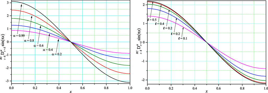
Numerical evaluation of x - ℓ RC D x + ℓ α sin π x for the fixed memory length ℓ = 0.2 (the left-hand side) and for the fixed value of order α = 0.6 (the right-hand side).

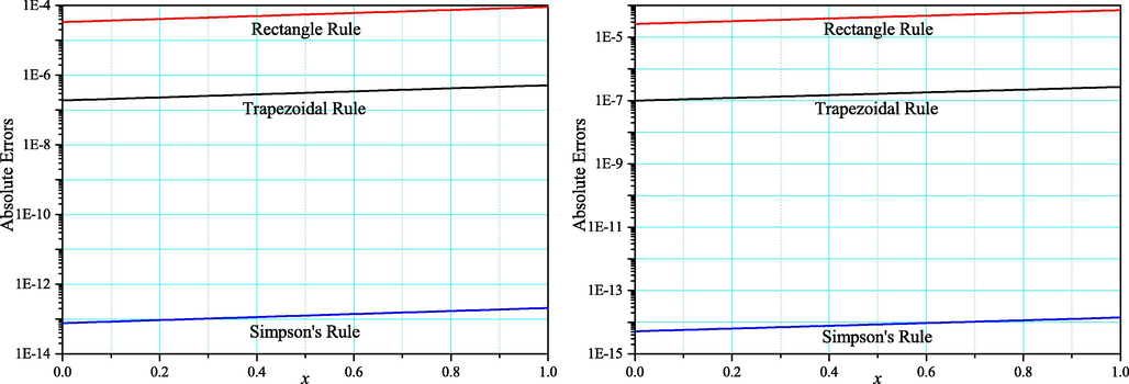
A semi-logarithmic plot of absolute errors generated by presented schemes for the Riesz–Caputo operator x - ℓ RC D x + ℓ α exp x for ℓ = 0.2 , Δ x = 0.002 , α = 0.6 (the left-hand side), and α = 1.2 (the right-hand side).

The results presented in Tables 1–3 show us that, in the case of RM and TM the rate ERC is close to 1 and 2, respectively, for each studied fractional operator. We see that the rate ERC depends on the order of the derivative $α$ for the left and right Caputo operators while for the Riesz–Caputo derivative it is close to 4. Moreover, the smallest errors are generated by Simpson’s rule, which is consistent with the classical theory of numerical integration.

Fig. 1 presents plots of the Riesz–Caputo derivative with the fixed memory length $ℓ$ of the function $\sin (π x)$ . Analyzing these results we can observe the influence of the order of the derivative $α$ and the fixed memory length $ℓ$ on the solution. Finally, Fig. 2 reveals (on a semi-logarithmic plot) how errors change in the interval $[0, 1]$ for the Riesz–Caputo derivative with fixed memory length $ℓ = 0.2$ of the function $\exp (x)$ and for each presented method. We conclude that the smallest errors are generated by PM while the largest errors are obtained for RM.

6 Conclusions

In this paper, a numerical approximation of the left and right Caputo derivatives and the Riesz–Caputo operator with fixed memory length has been proposed. The comparison of three modified methods of numerical approximation for selected fractional operators is presented. For the first time, the presented methods include the evaluation of considered fractional derivatives with fixed memory. The obtained numerical results are compared with the exact ones. The exact values were calculated by using the series representation of fractional operators with the fixed memory length. Absolute errors and the experimental rates of convergence were established. Our future research will focus on extending the proposed approach to operators of variable order. Moreover, the presented numerical schemes could be used to solve differential equations appearing in fractional continuum mechanics.

CRediT authorship contribution statement

Tomasz Blaszczyk: Software, Methodology, Validation, Formal analysis, Investigation, Writing - original draft, Writing - review & editing, Supervision. Krzysztof Bekus: Software, Validation, Formal analysis, Investigation, Writing - original draft, Writing - review & editing, Visualization. Krzysztof Szajek: Methodology, Investigation, Writing - original draft, Writing - review & editing. Wojciech Sumelka: Conceptualization, Methodology, Formal analysis, Investigation, Writing - original draft, Writing - review & editing, Funding acquisition, Supervision.

Acknowledgements

This work is supported by the National Science Centre, Poland under Grant No. 2017/27/B/ST8/00351

Declaration of Competing Interest

The authors declare that they have no known competing financial interests or personal relationships that could have appeared to influence the work reported in this paper.

References

Atanackovic T.M., Stankovic B., . Generalized wave equation in nonlocal elasticity. Acta Mechanica. 2009;208(1–2):1-10.
[Google Scholar]
Atangana A., Owolabi K.M., . New numerical approach for fractional differential equations. Mathematical Modelling of Natural Phenomena. 2018;13(1):3.
[Google Scholar]
Blaszczyk T., Leszczynski J., Szymanek E., . Numerical solution of composite left and right fractional Caputo derivative models for granular heat flow. Mechanics Research Communications. 2013;48:42-45.
[Google Scholar]
Blaszczyk T., Siedlecki J., Ciesielski M., . Numerical algorithms for approximation of fractional integral operators based on quadratic interpolation. Mathematical Methods in the Applied Sciences. 2018;41(9):3345-3355.
[Google Scholar]
Ciesielski M., Blaszczyk T., . The multiple composition of the left and right fractional Riemann-Liouville integrals – analytical and numerical calculations. Filomat. 2017;31(19):6087-6099.
[Google Scholar]
Dehghan M., Yousefi S.A., Lotfi A., . The use of He’s variational iteration method for solving the telegraph and fractional telegraph equations. International Journal for Numerical Methods in Biomedical Engineering. 2011;27(2):219-231.
[Google Scholar]
Diethelm K., . The analysis of fractional differential equations.Lecture Notes in Mathematics. Vol vol. 2004. Springer-Verlag; 2010.
Drapaca C.S., Sivaloganathan S., . A fractional model of continuum mechanics. Journal of Elasticity. 2012;107:107-123.
[Google Scholar]
Faraji Oskouie M., Ansari R., Rouhi H., . Vibration analysis of fg nanobeams on the basis of fractional nonlocal model: a variational approach. Microsystem Technologies. 2018;24(6):2775-2782.
[Google Scholar]
Gomez-Aguilar J.F., Saad K.M., Baleanu D., . Fractional dynamics of an erbium-doped fiber laser model. Optical and Quantum Electronics. 2019;51:316.
[Google Scholar]
Kilbas A.A., Srivastava H.M., Trujillo J.J., . Theory and Applications of Fractional Differential Equations. Amsterdam: Elsevier; 2006.
Lazopoulos A.K., . On fractional peridynamic deformations. Archive of Applied Mechanics. 2016;86(12):1987-1994.
[Google Scholar]
Lin Z., Wang D., . A finite element formulation preserving symmetric and banded diffusion stiffness matrix characteristics for fractional differential equations. Computational Mechanics. 2018;62(2):185-211.
[Google Scholar]
Machado J.A.T., Kiryakova V., Mainardi F., . Recent history of fractional calculus. Communications in Nonlinear Science and Numerical Simulation. 2011;16(3):1140-1153.
[Google Scholar]
Meerschaert M., Tadjeran Ch., . Finite difference approximations for two-sided space-fractional partial differential equations. Applied Numerical Mathematics. 2006;56(1):80-90.
[Google Scholar]
Miller M., Guy W. Jr., . Numerical inversion of the laplace transform by use of Jacobi polynomials. SIAM Journal on Numerical Analysis. 1966;3(4):624-635.
[Google Scholar]
Mustafa G., Yalcin O., Ayse A., . Numerical approach for solving fractional relaxation–oscillation equation. Applied Mathematical Modelling. 2013;37(8):5927-5937.
[Google Scholar]
Owolabi K.M., . Analysis and numerical simulation of multicomponent system with Atangana–Baleanu fractional derivative. Chaos, Solitons & Fractals. 2018;115:127-134.
[Google Scholar]
Podlubny, I. 1999. Fractional Differential Equations. Volume 198 of Mathematics in Science and Engineering. Academic Press.
Prakash A., Kumar M., Baleanu D., . A new iterative technique for a fractional model of nonlinear Zakharov–Kuznetsov equations via Sumudu transform. Applied Mathematics and Computation. 2018;334:30-40.
[Google Scholar]
Qureshi S., Kumar P., . Using Shehu integral transform to solve fractional order Caputo type initial value problems. Journal of Applied Mathematics and Computational Mechanics. 2019;18(2):75-83.
[Google Scholar]
Saad K.M., Deniz S., Baleanu D., . On a new modified fractional analysis of Nagumo equation. International Journal of Biomathematics. 2019;12(3):1950034.
[Google Scholar]
Saad, K.M., AL-Shareef, Eman. H.F., Alomari, A.K., Baleanu, D., Gomez-Aguilar, J.F., 2020. On exact solutions for time-fractional Korteweg-de Vries and Korteweg-de Vries-Burger’s equations using homotopy analysis transform method. Chinese Journal of Physics 63, 149–162.
Singh H., . Analysis for fractional dynamics of Ebola virus model, chaos solitons & fractals. Chaos, Solitons & Fractals. 2020;138:109992
[Google Scholar]
Singh H., . Numerical simulation for fractional delay differential equations. International Journal of Dynamics and Control 2020
[Google Scholar]
Singh H., Srivastava H.M., . Numerical simulation for fractional-order Bloch equation arising in nuclear magnetic resonance by using the Jacobi polynomials. Applied Sciences. 2020;10(8):2850.
[Google Scholar]
Singh H., Pandey R.K., Srivastava H.M., . Solving non-linear fractional variational problems using Jacobi polynomials. Mathematics. 2019;7(3):224.
[Google Scholar]
Singh H., Ghassabzadeh F.A., Tohidi E., Cattani C., . Legendre spectral method for the fractional Bratu problem. Mathematical Methods in the Applied Sciences. 2020;43(9):5941-5952.
[Google Scholar]
Sumelka W., . Thermoelasticity in the framework of the fractional continuum mechanics. Journal of Thermal Stresses. 2014;37(6):678-706.
[Google Scholar]
Sumelka W., . On fractional non-local bodies with variable length scale. Mechanics Research Communications. 2017;86(Supplement C):5-10.
[Google Scholar]
Sumelka W., Blaszczyk T., . Fractional continua for linear elasticity. Archives of Mechanics. 2014;66(3):147-172.
[Google Scholar]
Sumelka W., Voyiadjis G.V., . A hyperelastic fractional damage material model with memory. International Journal of Solids and Structures. 2017;124
[Google Scholar]
Sumelka W., Blaszczyk T., Liebold C., . Fractional euler–bernoulli beams: Theory, numerical study and experimental validation. European Journal of Mechanics - A/Solids. 2015;54:243-251.
[Google Scholar]
Szajek K., Sumelka W., Blaszczyk T., Bekus K., . On selected aspects of space-fractional continuum mechanics model approximation. International Journal of Mechanical Sciences. 2020;167
[Google Scholar]
Wei Y.H., Chen Y.Q., Cheng S.S., Wang Y., . A note on short memory principle of fractional calculus. Fractional Calculus and Applied Analysis. 2017;20(6):1382-1404.
[Google Scholar]
Yuan L., Agrawal O.P., . A numerical scheme for dynamic systems containing fractional derivatives. Computational Mechanics. 2019;63(4):713-723.
[Google Scholar]
Zhang X.-Y., Li X.-F., . Transient thermal stress intensity factors for a circumferential crack in a hollow cylinder based on generalized fractional heat conduction. International Journal of Thermal Sciences. 2017;121:336-347.
[Google Scholar]

Introduction

Preliminaries

Series representation of fractional operators with fixed memory length

Numerical schemes for Caputo derivatives

Approximation based on the rectangle rule
Approximation based on the trapezoidal rule
Approximation based on Simpson’s rule
Approximations of the Riesz–Caputo operator

Results

Conclusions

CRediT authorship contribution statement

Fulltext Views
39

PDF downloads
23

View/Download PDF
Download Citations

BibTeX
RIS

Show Sections

[1] Atanackovic T.M., Stankovic B., . Generalized wave equation in nonlocal elasticity. Acta Mechanica. 2009;208(1–2):1-10.
[Google Scholar]

[2] Atangana A., Owolabi K.M., . New numerical approach for fractional differential equations. Mathematical Modelling of Natural Phenomena. 2018;13(1):3.
[Google Scholar]

[3] Blaszczyk T., Leszczynski J., Szymanek E., . Numerical solution of composite left and right fractional Caputo derivative models for granular heat flow. Mechanics Research Communications. 2013;48:42-45.
[Google Scholar]

[4] Blaszczyk T., Siedlecki J., Ciesielski M., . Numerical algorithms for approximation of fractional integral operators based on quadratic interpolation. Mathematical Methods in the Applied Sciences. 2018;41(9):3345-3355.
[Google Scholar]

[5] Ciesielski M., Blaszczyk T., . The multiple composition of the left and right fractional Riemann-Liouville integrals – analytical and numerical calculations. Filomat. 2017;31(19):6087-6099.
[Google Scholar]

[6] Dehghan M., Yousefi S.A., Lotfi A., . The use of He’s variational iteration method for solving the telegraph and fractional telegraph equations. International Journal for Numerical Methods in Biomedical Engineering. 2011;27(2):219-231.
[Google Scholar]

[7] Diethelm K., . The analysis of fractional differential equations.Lecture Notes in Mathematics. Vol vol. 2004. Springer-Verlag; 2010.

[8] Drapaca C.S., Sivaloganathan S., . A fractional model of continuum mechanics. Journal of Elasticity. 2012;107:107-123.
[Google Scholar]

[9] Faraji Oskouie M., Ansari R., Rouhi H., . Vibration analysis of fg nanobeams on the basis of fractional nonlocal model: a variational approach. Microsystem Technologies. 2018;24(6):2775-2782.
[Google Scholar]

[10] Gomez-Aguilar J.F., Saad K.M., Baleanu D., . Fractional dynamics of an erbium-doped fiber laser model. Optical and Quantum Electronics. 2019;51:316.
[Google Scholar]

[11] Kilbas A.A., Srivastava H.M., Trujillo J.J., . Theory and Applications of Fractional Differential Equations. Amsterdam: Elsevier; 2006.

[12] Lazopoulos A.K., . On fractional peridynamic deformations. Archive of Applied Mechanics. 2016;86(12):1987-1994.
[Google Scholar]

[13] Lin Z., Wang D., . A finite element formulation preserving symmetric and banded diffusion stiffness matrix characteristics for fractional differential equations. Computational Mechanics. 2018;62(2):185-211.
[Google Scholar]

[14] Machado J.A.T., Kiryakova V., Mainardi F., . Recent history of fractional calculus. Communications in Nonlinear Science and Numerical Simulation. 2011;16(3):1140-1153.
[Google Scholar]

[15] Meerschaert M., Tadjeran Ch., . Finite difference approximations for two-sided space-fractional partial differential equations. Applied Numerical Mathematics. 2006;56(1):80-90.
[Google Scholar]

[16] Miller M., Guy W. Jr., . Numerical inversion of the laplace transform by use of Jacobi polynomials. SIAM Journal on Numerical Analysis. 1966;3(4):624-635.
[Google Scholar]

[17] Mustafa G., Yalcin O., Ayse A., . Numerical approach for solving fractional relaxation–oscillation equation. Applied Mathematical Modelling. 2013;37(8):5927-5937.
[Google Scholar]

[18] Owolabi K.M., . Analysis and numerical simulation of multicomponent system with Atangana–Baleanu fractional derivative. Chaos, Solitons & Fractals. 2018;115:127-134.
[Google Scholar]

[19] Podlubny, I. 1999. Fractional Differential Equations. Volume 198 of Mathematics in Science and Engineering. Academic Press.

[20] Prakash A., Kumar M., Baleanu D., . A new iterative technique for a fractional model of nonlinear Zakharov–Kuznetsov equations via Sumudu transform. Applied Mathematics and Computation. 2018;334:30-40.
[Google Scholar]

[21] Qureshi S., Kumar P., . Using Shehu integral transform to solve fractional order Caputo type initial value problems. Journal of Applied Mathematics and Computational Mechanics. 2019;18(2):75-83.
[Google Scholar]

[22] Saad K.M., Deniz S., Baleanu D., . On a new modified fractional analysis of Nagumo equation. International Journal of Biomathematics. 2019;12(3):1950034.
[Google Scholar]

[23] Saad, K.M., AL-Shareef, Eman. H.F., Alomari, A.K., Baleanu, D., Gomez-Aguilar, J.F., 2020. On exact solutions for time-fractional Korteweg-de Vries and Korteweg-de Vries-Burger’s equations using homotopy analysis transform method. Chinese Journal of Physics 63, 149–162.

[24] Singh H., . Analysis for fractional dynamics of Ebola virus model, chaos solitons & fractals. Chaos, Solitons & Fractals. 2020;138:109992
[Google Scholar]

[25] Singh H., . Numerical simulation for fractional delay differential equations. International Journal of Dynamics and Control 2020
[Google Scholar]

[26] Singh H., Srivastava H.M., . Numerical simulation for fractional-order Bloch equation arising in nuclear magnetic resonance by using the Jacobi polynomials. Applied Sciences. 2020;10(8):2850.
[Google Scholar]

[27] Singh H., Pandey R.K., Srivastava H.M., . Solving non-linear fractional variational problems using Jacobi polynomials. Mathematics. 2019;7(3):224.
[Google Scholar]

[28] Singh H., Ghassabzadeh F.A., Tohidi E., Cattani C., . Legendre spectral method for the fractional Bratu problem. Mathematical Methods in the Applied Sciences. 2020;43(9):5941-5952.
[Google Scholar]

[29] Sumelka W., . Thermoelasticity in the framework of the fractional continuum mechanics. Journal of Thermal Stresses. 2014;37(6):678-706.
[Google Scholar]

[30] Sumelka W., . On fractional non-local bodies with variable length scale. Mechanics Research Communications. 2017;86(Supplement C):5-10.
[Google Scholar]

[31] Sumelka W., Blaszczyk T., . Fractional continua for linear elasticity. Archives of Mechanics. 2014;66(3):147-172.
[Google Scholar]

[32] Sumelka W., Voyiadjis G.V., . A hyperelastic fractional damage material model with memory. International Journal of Solids and Structures. 2017;124
[Google Scholar]

[33] Sumelka W., Blaszczyk T., Liebold C., . Fractional euler–bernoulli beams: Theory, numerical study and experimental validation. European Journal of Mechanics - A/Solids. 2015;54:243-251.
[Google Scholar]

[34] Szajek K., Sumelka W., Blaszczyk T., Bekus K., . On selected aspects of space-fractional continuum mechanics model approximation. International Journal of Mechanical Sciences. 2020;167
[Google Scholar]

[35] Wei Y.H., Chen Y.Q., Cheng S.S., Wang Y., . A note on short memory principle of fractional calculus. Fractional Calculus and Applied Analysis. 2017;20(6):1382-1404.
[Google Scholar]

[36] Yuan L., Agrawal O.P., . A numerical scheme for dynamic systems containing fractional derivatives. Computational Mechanics. 2019;63(4):713-723.
[Google Scholar]

[37] Zhang X.-Y., Li X.-F., . Transient thermal stress intensity factors for a circumferential crack in a hollow cylinder based on generalized fractional heat conduction. International Journal of Thermal Sciences. 2017;121:336-347.
[Google Scholar]

On numerical approximation of the Riesz–Caputo operator with the fixed/short memory length

Abstract

Keywords

Fractional derivatives

Numerical schemes

Caputo operator

Riesz–Caputo operator

Fixed memory length

1 Introduction

2 Preliminaries

3 Series representation of fractional operators with fixed memory length

Theorem 1 Theorem 3.2 in Wei et al., 2017

Theorem 3 Theorem 3.1 in Wei et al., 2017

4 Numerical schemes for Caputo derivatives

4.1 Approximation based on the rectangle rule

4.2 Approximation based on the trapezoidal rule

4.3 Approximation based on Simpson’s rule

4.4 Approximations of the Riesz–Caputo operator

5 Results

6 Conclusions

CRediT authorship contribution statement

Acknowledgements

Declaration of Competing Interest

References

Suggested read for related articles: