On Marangoni shear convective flows of inhomogeneous viscous incompressible fluids in view of the Soret effect

1 Introduction

The Marangoni effect is a flow that occurs in a fluid under the effect surface tension difference. The Marangoni flow observed in colloid chemistry and hydrodynamics is directed from the region of low surface tension to the region of high surface tension. The effect is named after C. Marangoni and his research (Marangoni, 1865). Marangoni convection flows in a water column, visualized with the use of particle tracers, were repeatedly observed in experiments (Kim et al, 2017; Birikh et al, 2011).

It is known that the occurrence of a surface tension gradient can be caused by a temperature gradient or a concentration gradient. Diffusive instability associated with molecular exchange processes becomes important when studying the mechanisms of impurity transfer in a seawater fluid. Soret was one of the first to investigate salt transfer due to a thermal gradient (Soret, 1879). Due to the presence of a geothermal gradient in hydrocarbon deposits, the Soret effect has a significant effect on the formation of the geological profile (Ghorayeb et al., 2003). The opposite effect (the Dufour effect) (Dufour, 1872), which consists in the occurrence of a temperature difference in a fluid mixture due to a difference in the concentrations of the mixture components, is often ignored. This is explained by the fact that, in most cases, the Dufour effect is so small that it is neglected in the study of the flow of binary fluids (Demirel, 2007; Ortiz de Zárate and Sengers, 2006).

The Marangoni effect has a great influence on the formation of the morphology of thin films. The relevance of this line of a research is confirmed, for example, by (Fowler et al., 2016: Gupta and Tiwari, 2017; Mikishev et al., 2017). These studies are either experimental or use numerical calculations to analyze the properties of the films. The present paper is a theoretical study of the exact (analytical) solution of the Navier-Stokes equations which describes the effect of the superposition of inhomogeneous temperature and concentration fields on a viscous binary fluid flow in a horizontal layer of constant thickness, with the Marangoni effect taken into account. However, despite the fact that the exact solution presented in the paper is able to describe the flow of a viscous fluid in thin films, the main purpose of the study is somewhat different. The objective of the study is to obtain, based on the constructed exact solution, functional dependencies or estimates for the parameters of the boundary value problem, which would allow us to control the flow characteristics, for example, varying the parameters of layer heating or layer thickness in order to avoid/guarantee the occurrence of counterflows in the fluid.

The description of two-dimensional and three-dimensional thermal diffusion flows in the exact formulation is only beginning to develop. The paper (Aristov and Prosviryakov, 2016) proposes a class of exact solutions for studying the nonlinear properties of three-dimensional flows of binary fluids. To date, exact solutions for the description of unidirectional Marangoni flows $\left(V_x,0,0\right)$ of binary fluids (Andreev and Ryzhkov, 2013; Bekezhanova, 2011) and their stability have been investigated.

Exact solutions announced in (Andreev and Ryzhkov, 2013; Bekezhanova, 2011) belong to the Birikh class of exact solutions (Birikh, 1966). The exact Birikh solution is the first exact solution to the Oberbeck-Boussinesq equations. This solution describes thermocapillary convection in an infinite fluid layer. A generalization of the exact Birikh solution in the description of layered convective Marangoni flows $\left(V_x,V_y,0\right)$ is given in (Aristov and Prosviryakov, 2013; Aristov et al, 2016). The study of concentration convection for the velocity field $\left(V_x,V_y,0\right)$ is published in the article (Aristov et al, 2015).

However, to date, we are not aware of studies in the exact formulation of two-dimensional layered Marangoni flows $\left(V_x,V_y,0\right)$ of a binary fluid taking into account the dissipative Soret effect. The article presents an exact solution eliminating this drawback.

The manuscript material is divided into several sections. In the Problem Statement section, the basic equations of the model are given and the necessary notation is introduced. The Solution Class section describes the structure of the class of exact solutions for hydrodynamic fields, provides a general solution to the system of governing equations. In the Setting a Heat Source on the Upper Boundary of the Layer section, a boundary value problem describing convection of a viscous incompressible fluid induced by taking into account the Marangoni effect is formulated; a solution to the boundary value problem is given. The Analysis of the Flow Properties section analyzes in detail the properties of the flow velocity field and the shear stress field. In the Analysis of the Temperature Field and the Concentration Field section, the properties of the temperature and concentration fields are analyzed, and the corresponding profiles are constructed. The Analysis of the Pressure Field section describes the main properties of the pressure field, and its profile is given.

2 Problem statement

Let us consider a fluid mixture of two components. We assume that the mixture is in the field of gravity $\left(0,0,-g\right)$. Then the equations of the motion of a binary mixture in the Boussinesq approximation, describing the flow of a stratified viscous incompressible fluid, are written as follows (Gershuni and Zhukhovitskii, 1976):

In the system of Eq. (1), the following notations are introduced: $\mathit{V}=\left(V_x,V_y,V_z\right)$ is a velocity vector; $P\left(t,x,y,z\right)$ is the deviation of pressure from hydrostatic, divided by constant average density; $C\left(t,x,y,z\right)$ is the deviation of the concentration (salinity) of the light component of the mixture from the average value; $T\left(t,x,y,z\right)$ is deviation from the average temperature; $\nu$, $\chi$, $d$, $\alpha d$, ${\beta }_1$ and ${\beta }_2$ are the coefficients of kinematic viscosity, thermal diffusivity, diffusion, thermal diffusion, thermal and concentration expansion of the fluid, respectively.

The first three equations of system (1) are the projections of the vector equation of motion of a viscous fluid (Navier-Stokes equations) on the axis of the selected Cartesian coordinate system with allowance made for the Boussinesq approximation (Gershuni and Zhukhovitskii, 1976). The following two equations of system (1) are the heat equation and the concentration equation taking into account the Soret effect (Soret, 1879). The last equation of system (1) is the incompressibility equation.

For many engineering problems, flows in a round pipe (Batchelor, 2000; Gershuni and Zhukhovitskii, 1976), a flat channel or the boundary layer on a flat plate (Israelachvili et al., 1988; Savenkov, 2012), flows in a flat or axisymmetric wake behind a streamlined ball or cylinder (Isaev et al., 2007; Okhotnikov et al., 2017), as well as some other flows, are of great importance. All these classes of currents qualify as shear flows (Schmid and Henningson, 2001; Nasiruddin and Kamran, 2010; Fernandes, 2011).

When a steady motion in a shear fluid flow ($V_z=0$) is considered, system (1) is converted to the form$$V_x\frac{\partial V_x}{\partial x}+V_y\frac{\partial V_x}{\partial y}=-\frac{\partial P}{\partial x}+\nu \left(\frac{{\partial }^2{V}_x}{\partial x^2}+\frac{{\partial }^2{V}_x}{\partial y^2}+\frac{{\partial }^2{V}_x}{\partial z^2}\right),$$$$V_x\frac{\partial V_y}{\partial x}+V_y\frac{\partial V_y}{\partial y}=-\frac{\partial P}{\partial y}+\nu \left(\frac{{\partial }^2{V}_y}{\partial x^2}+\frac{{\partial }^2{V}_y}{\partial y^2}+\frac{{\partial }^2{V}_y}{\partial z^2}\right),$$$$\frac{\partial P}{\partial z}=g\left({\beta }_{1}T+{\beta }_{2}C\right),$$

In addition, the unknown hydrodynamic fields P, C, T and the components of the velocity vector $\mathit{V}$ become independent of time $t$.

3 Solution class

System (2) is nonlinear and overdetermined, since it consists of six equations for five unknown functions. The choice of a special class of exact solutions will allow us to reduce the number of equations of the system in question by identically satisfying a number of equations involved in it. For the solvability of this overdetermined system, the solution of equations (2) will be sought in the following form (Aristov and Shvarts, 2006; Aristov and Prosviryakov, 2016; Prosviryakov, 2019):$$V_x=U\left(z\right),V_y=V\left(z\right),P\left(x,y,z\right)=P_0\left(z\right)+P_1\left(z\right)x+P_2\left(z\right)y,$$

Note that the velocity field of the form (3) was first considered by Ekman (Ekman, 1905). Convective flows of the form as in Eq. (3) with constant horizontal temperature gradients ($T_1=const$, $T_2=const$) were first considered by Birikh (1966) and Ostroumov (1958). The effect of concentration on flow characteristics was investigated in Ryzhkov (2006); Ryzhkov and Shevtsova (2009); Andreev and Efimova (2018). The class of solutions represented by Eq. (3) was also investigated in Aristov and Prosviryakov (2013); Burmasheva and Prosviryakov (2017a, 2017b); Knyazev (2011); Schwarz (2014).

As a result of the substitution of the exact solution (3) into system (2), we obtain the system of equations$$\nu \frac{{\partial }^{2}U}{\partial z^2}=P_1,\nu \frac{{\partial }^{2}V}{\partial z^2}=P_2,$$$$\frac{\partial P_0}{\partial z}+\frac{\partial P_1}{\partial z}x+\frac{\partial P_2}{\partial z}y=g\left({\beta }_1{T}_0+{\beta }_2{C}_0+\left({\beta }_1{T}_1+{\beta }_2{C}_1\right)x+\left({\beta }_1{T}_2+{\beta }_2{C}_2\right)y\right),$$$$U{T}_1+V{T}_2=\chi \left(\frac{{\partial }^2{T}_0}{\partial z^2}+\frac{{\partial }^2{T}_1}{\partial z^2}x+\frac{{\partial }^2{T}_2}{\partial z^2}y\right),$$$$U{C}_1+V{C}_2=d\left(\frac{{\partial }^2{C}_0}{\partial z^2}+\frac{{\partial }^2{C}_1}{\partial z^2}x+\frac{{\partial }^2{C}_2}{\partial z^2}y\right)+\alpha d\left(\frac{{\partial }^2{T}_0}{\partial z^2}+\frac{{\partial }^2{T}_1}{\partial z^2}x+\frac{{\partial }^2{T}_2}{\partial z^2}y\right).$$

This system, due to the principle of undetermined coefficients, is equivalent to the system$$\frac{{\partial }^2{T}_1}{\partial z^2}=0,\frac{{\partial }^2{T}_2}{\partial z^2}=0,\frac{{\partial }^2{C}_1}{\partial z^2}=0,\frac{{\partial }^2{C}_2}{\partial z^2}=0,$$$$\frac{\partial P_1}{\partial z}=g\left({\beta }_1{T}_1+{\beta }_2{C}_1\right),\frac{\partial P_2}{\partial z}=g\left({\beta }_1{T}_2+{\beta }_2{C}_2\right),$$

The equations are written in the order of integration of system (4). The general solution of system (4) is$$C_1=c_{1}z+c_2,C_2=c_{3}z+c_4,T_1=c_{5}z+c_6,$$$$P_1=g\left(\frac{{\beta }_1{c}_5+{\beta }_2{c}_1}{2}{z}^2+\left({\beta }_1{c}_6+{\beta }_2{c}_2\right)z\right)+c_7,T_2=c_{8}z+c_9,$$$$P_2=g\left(\frac{{\beta }_1{c}_8+{\beta }_2{c}_3}{2}{z}^2+\left({\beta }_1{c}_9+{\beta }_2{c}_3\right)z\right)+c_{10},$$$$U=\frac{\left({\beta }_1{c}_5+{\beta }_2{c}_1\right)z^4+4\left({\beta }_1{c}_6+{\beta }_2{c}_2\right)z^3+12c_7{z}^2+24\nu c_{11}z}{24\nu }+c_{12},$$$$V=\frac{\left({\beta }_1{c}_8+{\beta }_2{c}_3\right)z^4+4\left({\beta }_1{c}_9+{\beta }_2{c}_4\right)z^3+12c_{10}{z}^2+24\nu c_{13}z}{24\nu }+c_{14}.$$

To find the integration constants $c_i$, where $i=\overline{1,19}$, in the general solution of system (4), we formulate boundary conditions. Convective fluid flows with a specified heat source at one or both boundaries of a horizontal infinite layer were discussed in Aristov and Prosviryakov (2013). In the simulation of thermal diffusion flows, the solution of system (4) becomes much more complicated. When the heat flux is set at one boundary, the change of the concentration can be implemented both at one boundary and at both boundaries.

4 Setting a heat source on the upper boundary of the layer

Let us study the flow of a stratified viscous incompressible fluid in an infinite horizontal layer of thickness h (Fig. 1), for which the influence of thermocapillary forces on the free boundary is significant.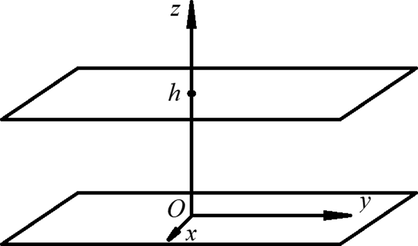

Close

Fig. 1

The geometry of the flow.

Export to PPT

We assume that the lower boundary $z=0$ is rigid and that the no-slip condition is given. The boundary $z=0$ is isothermal, the concentration value on it being taken as the reference (zero) value. At the free rigid upper boundary, temperature and concentration are specified, with capillary forces induced by the presence of a temperature gradient acting there. The pressure at the upper boundary is assumed to be equal to the atmospheric pressure. In this case, the stationary boundary conditions have the form

Here, $\eta$ is the dynamic viscosity coefficient; the surface tension coefficient $\alpha$ is assumed to be linearly dependent on temperature and concentration (Gershuni and Zhukhovitskii, 1976),$$\alpha ={\sigma }_0-{\sigma }_{1}T-{\sigma }_{2}C,$$where ${\sigma }_1$ and ${\sigma }_2$ are the temperature and concentration surface tension coefficients, respectively. Taking into account the structure of the exact solution (2), this dependence takes the form$$\alpha ={\sigma }_0-{\sigma }_{1}T-{\sigma }_{2}C={\sigma }_0-{\sigma }_1\left(T_0+T_{1}x+T_{2}y\right)-{\sigma }_2\left(C_0+C_{1}x+C_{2}y\right).$$

Considering the structure of the class of solutions (3), the boundary conditions represented by Eq. (5) at the lower boundary take the form

Similarly, the conditions on the upper boundary are written as

Note that in the notation of the boundary conditions (6), (7) there is an ambiguity in the interpretation of the symbol C. It is used for both the concentration field and the value of its longitudinal gradient at the upper boundary. Hereinafter, the symbol C is used only for the horizontal concentration gradient. The boundary conditions as in Eq. (7) for concentration convection (${\sigma }_1=0$) or for thermocapillary convection (${\sigma }_2=0$) were considered in Aristov et al. (2015, 2016)); Vakulenko and Sudakov (2016).

We next introduce a dimensionless variable $Z=z/h\in \left[0,1\right]$ (h is the thickness of the fluid layer under consideration). Then, taking into account this substitution, the exact solution of the boundary value problem (4), (6–7) takes the form$$T_1=AZ,T_2=BZ,C_1=CZ,C_2=DZ,$$$$U=-{\gamma }_{1}Z+{\gamma }_2\left(Z^4-6Z^2+8Z\right),V=-{\gamma }_{3}Z+{\gamma }_4\left(Z^4-6Z^2+8Z\right),$$$$P_1=\frac{g\eta }{2}{\gamma }_1\left(Z^2-1\right),P_2=\frac{g\eta }{2}{\gamma }_3\left(Z^2-1\right),$$

Here, we introduce the following notations for the coefficients:$${\gamma }_1=\left(A{\sigma }_1+C{\sigma }_2\right)\frac{h}{\eta },{\gamma }_2=\frac{g{h}^3}{24\nu }\left(A{\beta }_1+C{\beta }_2\right),{\gamma }_3=\left(B{\sigma }_1+D{\sigma }_2\right)\frac{h}{\eta },{\gamma }_4=\frac{g{h}^3}{24\nu }\left(B{\beta }_1+D{\beta }_2\right),$$$${\psi }_1=\frac{g{h}^5}{5040\nu \chi }\left(\left(A^2+B^2\right){\beta }_1+\left(\mathit{AC}+BD\right){\beta }_2\right),{\psi }_2=\frac{\left(\left(A^2+B^2\right){\sigma }_1+\left(\mathit{AC}+BD\right){\sigma }_2\right)h^3}{12\eta \chi },$$$${\psi }_3=\frac{g{h}^5}{5040\nu }\left(\left(\mathit{AC}+BD\right)\left(\frac{{\beta }_1}{d}-\frac{\alpha {\beta }_2}{\chi }\right)-\left(A^2+B^2\right)\frac{\alpha {\beta }_1}{\chi }+\left(C^2+D^2\right)\frac{{\beta }_2}{d}\right),$$$${\psi }_4=\frac{h^3}{12\eta }\left(\left(\mathit{AC}+BD\right)\left({\sigma }_1+\alpha {\sigma }_2\right)-\left(A^2+B^2\right)\alpha {\sigma }_1-\left(C^2+D^2\right){\sigma }_2\right),$$$${\psi }_5=\frac{1}{40320}\left[\frac{g^2{\beta }_1}{\nu \chi h^2}\left(\left(A^2+B^2\right){\beta }_1+\left(\mathit{AC}+BD\right){\beta }_2\right)+\right.$$$$\left.+\frac{g^2{\beta }_1}{\nu h^2}\left(\left(\mathit{AC}+BD\right)\left(\frac{{\beta }_1}{d}-\frac{\alpha {\beta }_2}{\chi }\right)-\left(A^2+B^2\right)\frac{\alpha {\beta }_1}{\chi }+\left(C^2+D^2\right)\frac{{\beta }_2}{d}\right)\right],$$$${\psi }_6=\frac{g{h}^4}{1440\eta }\left[\frac{{\beta }_{1}h}{\chi }\left(\left(A^2+B^2\right){\sigma }_1+\left(\mathit{AC}+BD\right){\sigma }_2\right)+\right.$$$$\left.+{\beta }_2\left(\left(\mathit{AC}+BD\right)\left({\sigma }_1+\alpha {\sigma }_2\right)-\left(A^2+B^2\right)\alpha {\sigma }_1-\left(C^2+D^2\right){\sigma }_2\right)\right].$$

The exact solution (8) of the stated boundary problem can be simplified if the equalities$$\frac{B}{A}=\frac{D}{C}=k$$

are simultaneously fulfilled, i.e. there is a rotation mapping $tg\phi =k$, which makes it possible to reduce the dimension of the problem in question since, in this case, according to the exact solution (8), the velocity $V$ takes the form$$V=-{\gamma }_{3}Z+{\gamma }_4\left(Z^4-6Z^2+8Z\right)=-k{\gamma }_{1}Z+k{\gamma }_2\left(Z^4-6Z^2+8Z\right)=kU.$$

Thus, the dimension of the boundary value problem (4), (6–7) will be equal to “one and a half”. It should be noted that, in contrast to thermal convection (Burmasheva and Prosviryakov, 2017a, 2017b, 2017c), this rotation mapping should take into account the cross-dissipative effects. Thus, the possibility of the reducing the dimension of the thermal diffusion problem under study is a rarer event than that for convective currents (Aristov and Prosviryakov, 2013) induced only by non-uniform temperature distribution.

Besides, the dimension can be reduced by rotation in two particular cases:

$A^2+B^2=0$, $D=kC$ and $C^2+D^2=0$, $B=kA$ (here $k\ne 0$,).

It is easy to show that, by virtue of Eq. (8), the horizontal velocities will become proportional in both cases,$$V=kU.$$

Moreover, the existence of the corresponding rotation mapping requires the agreement among the parameters describing only one type of the convection – either concentrational or thermal. Note that, in the case of a unidirectional flow, it is also possible to reduce the dimension in the analysis of other hydrodynamic fields,$$T_2=k{T}_1,P_2=k{P}_1,C_2=k{C}_1.$$

5 Analysis of the flow properties

Let us study the properties of the convective flow of an inhomogeneous viscous incompressible fluid. We analyze in detail the properties of the velocity $V_x=U$ represented as

If ${\gamma }_2=0$, which is equivalent to the condition $A{\beta }_1+C{\beta }_2=0$, Eq. (9) for the velocity $U$ will be significantly simplified to$$U=-{\gamma }_{1}Z.$$

In this case, the velocity $U$ describes the Couette-type flow (Couette, 1890) in the direction of the axis $\mathit{Ox}$. The velocity will be non-zero everywhere inside the layer. The flow will maintain the direction of motion relative to the axis $\mathit{Ox}$, and its velocity will increase linearly as it moves away from the lower boundary of the layer. There are no stagnant points for this velocity. The profile of the velocity $U$ is a segment of the axis passing through the origin. Note that, in the general case, the velocity in the direction of the axis $\mathit{Oy}$ can remain essentially nonlinear. The analysis of this particular case is of no interest; therefore, we will further assume that ${\gamma }_2\ne 0$.

In view of the fact that the bracketed terms in Eq. (9) define a strictly monotonic function, the velocity $U$ can have only one critical (zero) point, the necessary and sufficient condition for its existence being the fulfillment of the inequality$$\left(-{\gamma }_1+8{\gamma }_2\right)\left(-{\gamma }_1+3{\gamma }_2\right)<0.$$

We divide both sides of this inequality by ${\left({\gamma }_2\right)}^2\ne 0$; herewith, the inequality sign remains unchanged, i.e.$$\left(\frac{{\gamma }_1}{{\gamma }_2}-8\right)\left(\frac{{\gamma }_1}{{\gamma }_2}-3\right)<0.$$

The resulting inequality is equivalent to the condition$$3<\frac{{\gamma }_1}{{\gamma }_2}<8,$$under which the velocity field is stratified into two zones. In the fluid layer there appear two streams moving in different directions. These streams can be observed at the arbitrarily signed values of the horizontal temperature gradient A and the concentration gradient C given on $z=h$, even for abnormal fluids (${\sigma }_1<0$).

Rewrite Eq. (8) for velocity in the form

With this factorization of the expression for the velocity U, the parameter ${\gamma }_2$ does not affect the qualitative behavior of the velocity profile at a particular relation ${\gamma }_1/{\gamma }_2$, but it determines only the coefficient of stretching or compression of this profile relative to the transverse axis $\mathit{OZ}$. The dependence of the profiles on the parameter ${\gamma }_1/{\gamma }_2$ is shown in Fig. 2. Note that the larger the ratio ${\gamma }_1/{\gamma }_2$ in the absolute value, the closer to the lower boundary is the point of intersection of the velocity profile with the transverse coordinate axis.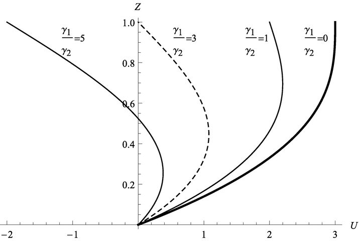

Close

Fig. 2

The dependence of the velocity profile shape on the parameter ${\gamma }_1/{\gamma }_2$ (the parameters ${\gamma }_1$, ${\gamma }_2$ are the coefficients of the exact solution (8)).

Export to PPT

The presence of a return section on the velocity hodograph (Fig. 3) indicates that the exact solution (8) describes the locally spiral flow of an inhomogeneous viscous incompressible fluid caused by the vortices moving in the layer relative to the axes 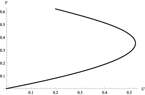$\mathit{Ox}$ and $\mathit{Oy}$.

Close

Fig. 3

The velocity vector hodograph at ${\gamma }_1=-1$, ${\gamma }_2={\gamma }_4=-0.4$, ${\gamma }_3=5$ (the parameters ${\gamma }_1$, ${\gamma }_2$, ${\gamma }_4$, ${\gamma }_5$ are the coefficients of the exact solution (8)).

Export to PPT

The dependence of the vertical coordinate, which determines the stagnant point (the boundary of the interaction of the streams), on the control parameters ${\gamma }_1/{\gamma }_2$ is shown in Fig. 4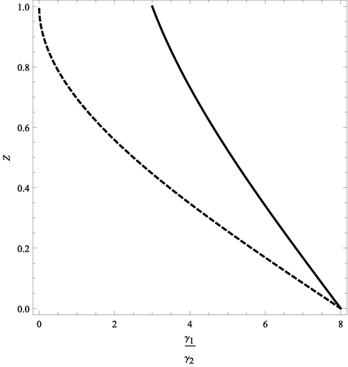

Close

Fig. 4

The dependence of the coordinates of the stagnant points of the velocity $U$ (solid line) and the tangential stress ${\tau }_{\mathit{xz}}$ (dashed line) on the control parameters ${\gamma }_1/{\gamma }_2$ (the parameters ${\gamma }_1$, ${\gamma }_2$ are the coefficients of the exact solution (8)).

Export to PPT

Note that the components$${\mathrm{\Omega }}_x=-\frac{1}{h}\frac{\mathit{dV}}{\mathit{dZ}},{\mathrm{\Omega }}_y=\frac{1}{h}\frac{\mathit{dU}}{\mathit{dZ}}$$of the vorticity vector $\mathrm{\Omega }=rot\mathit{V}$ calculated for the class (3) with an accuracy of a constant multiplier coincide with the corresponding tangential stress,$${\tau }_{\mathit{xz}}=\eta \frac{\mathit{dU}}{\mathit{dz}}=\frac{\eta }{h}\frac{\mathit{dU}}{\mathit{dZ}}=\frac{\eta }{h}\left(-{\gamma }_1+{\gamma }_2\left(4Z^3-12Z+8\right)\right)=\frac{4{\gamma }_2\eta }{h}\left(Z^3-3Z+2-\frac{{\gamma }_1}{4{\gamma }_2}\right),$$

The derivative of the polynomial $f\left(Z\right)=Z^3-3Z$ in the expressions for the velocities $U$ and $V$ is $f^{\prime }\left(Z\right)=3\left(Z^2-1\right)$, and it does not vanish anywhere in the layer. Therefore, according to Eq. (11), the tangential stresses ${\tau }_{\mathit{xz}}$ and ${\tau }_{\mathit{yz}}$ are determined by strictly monotonic functions on the interval $\left[0,1\right]$. Consequently, by analogy with the reasoning given for the velocity $U$, the tangential stresses can vanish inside the layer at no more than one value of the height $Z_0$ each. This means that, in view of the relation of the stresses ${\tau }_{\mathit{xz}}$ and ${\tau }_{\mathit{yz}}$ to the components ${\mathrm{\Omega }}_x$ and ${\mathrm{\Omega }}_y$ inside the layer, there can exist a thickness $h_0$ at which the vortices change their direction. The stress ${\tau }_{\mathit{xz}}$ vanishes inside the layer when the condition$$0<\frac{{\gamma }_1}{{\gamma }_2}<8$$is satisfied.

Thus, if the velocity $U$ has a critical point, there is $Z_0$, which corresponds to the interface between the tensile and compressive stresses ${\tau }_{\mathit{xz}}$. The converse is not true in the general case.

From Eq. (11) for the stress ${\tau }_{\mathit{xz}}$, we easily obtain an equation satisfied by the coordinate corresponding to the boundary between the areas of tensile and compressive stresses,$$Z^3-3Z+2-\frac{{\gamma }_1}{4{\gamma }_2}=0.$$

The dependence of this coordinate on the control parameters is presented in Fig. 4.

Fig. 4, in particular, illustrates that the tangential stress ${\tau }_{\mathit{xz}}$ and the longitudinal velocity $U$ never vanish simultaneously inside the layer.

Solving Eqs. (11) with respect to $h$, we can find the layer thickness at which the tangential stresses ${\tau }_{\mathit{xz}}$ and ${\tau }_{\mathit{yz}}$ vanish at any arbitrarily chosen height $Z$. As an example, consider the lower boundary $Z=0$ of the layer. The tangential stresses at the lower boundary, according to Eq. (11), are determined by the expressions$${\left.{\tau }_{\mathit{xz}}\right|}_{Z=0}=\frac{\eta }{h}\left(-{\gamma }_1+8{\gamma }_2\right)=-\left(A{\sigma }_1+C{\sigma }_2\right)+\frac{g{h}^2\rho }{3}\left(A{\beta }_1+C{\beta }_2\right),$$$${\left.{\tau }_{\mathit{yz}}\right|}_{Z=0}=\frac{\eta }{h}\left(-{\gamma }_3+8{\gamma }_4\right)=-\left(B{\sigma }_1+D{\sigma }_2\right)+\frac{g{h}^2\rho }{3}\left(B{\beta }_1+D{\beta }_2\right).$$

Accordingly, they vanish if$$h_1=\sqrt{\frac{3\left(A{\sigma }_1+C{\sigma }_2\right)}{g\rho \left(A{\beta }_1+C{\beta }_2\right)}},h_2=\sqrt{\frac{3\left(B{\sigma }_1+D{\sigma }_2\right)}{g\rho \left(B{\beta }_1+D{\beta }_2\right)}}.$$

At the same time, the tangential stresses vanish when $h_1$ and $h_2$ coincide, i.e. when $B/A=D/C\ne 0$.

We now determine the conditions under which the flow will become potential. For the flow to became irrotational, it is necessary that the projections ${\mathrm{\Omega }}_x$ and ${\mathrm{\Omega }}_y$, or, equivalently, the tangential stresses ${\tau }_{\mathit{xz}}$ and ${\tau }_{\mathit{yz}}$, vanish simultaneously. It is possible only when$$\frac{{\gamma }_1}{{\gamma }_2}=\frac{{\gamma }_3}{{\gamma }_4}.$$

That is, only when the equality $B/A=D/C$ is valid; as noted above, this equality implies the existence of the rotation mapping, which allows one to reduce the dimension of the problem. In this case, the corresponding tangential stress vanishes at no more than one point.

6 Analysis of the temperature field and the concentration field

According to the exact solution (8), the solution structure for the temperature field components completely (up to a difference in the coefficients) repeats the solution structure for the concentration field components. Therefore, conclusions regarding the properties of the temperature field can be easily extended to the properties of the concentration field.

It is obvious that the horizontal (longitudinal) temperature gradients $T_1$ and $T_2$ are strictly monotonic functions, which take only values of the same sign in the horizontal layer under study. The sign of the components $T_1$ and $T_2$ is determined by the values $A$ and $B$ taken by these gradients at the upper boundary of the layer. In what follows, we consider the properties of the background temperature $T_0$.

If the parameters of the boundary value problem are such that $\left(A^2+B^2\right){\sigma }_1+\left(\mathit{AC}+BD\right){\sigma }_2=0$ (i.e. ${\psi }_2=0$), the background temperature is described by the expression$$T_0={\psi }_1\left(5Z^7-63Z^6+140Z^4-82Z\right).$$

This means that, for any (nonzero) value of the coefficient ${\psi }_1$, the background temperature $T_0$ cannot be stratified into zones relative to the reference value (Fig. 5, dashed line).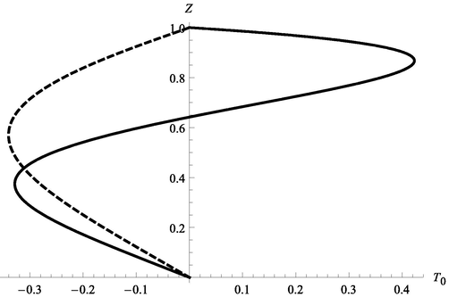

Close

Fig. 5

The profile of the background temperature $T_0$ at ${\psi }_1=0.01$, ${\psi }_2=0$ (dashed line) and at ${\psi }_1=0.1$, ${\psi }_2=7$ (solid line) (the parameters ${\psi }_1$, ${\psi }_2$ are the coefficients of the exact solution (8)).

Export to PPT

If the coefficient ${\psi }_2$ is nonzero, then, for some combinations of parameters, the background temperature can take a zero (reference) value inside the layer under consideration (Fig. 5, solid line). Moreover, the position of the zero point depends on the ratio ${\psi }_1$/${\psi }_2$.

Thus, the background concentration C₀ can also be stratified into two zones, in one of which the impurity concentration exceeds the reference value, and in the other it is below it (Fig. 6).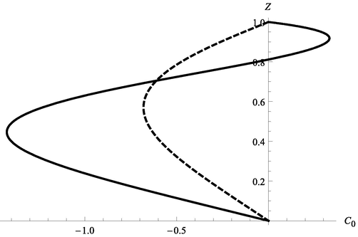

Close

Fig. 6

The profile of the background concentration C₀ at ${\psi }_3=0.02$, ${\psi }_4=0$ (dashed line) and ${\psi }_3=0.2$, ${\psi }_4=12$ (solid line) (the parameters ${\psi }_3$, ${\psi }_4$ are the coefficients of the exact solution (8)).

Export to PPT

7 Analysis of the pressure field

The longitudinal gradients $P_1$ and $P_2$ of the pressure field, as well as the longitudinal gradients of the temperature and concentration fields, are monotonic functions according to the exact solution (8). The background pressure $P_0$ is determined by the interaction of two terms, each of which is described by a high-degree polynomial. Depending on the ratio of the coefficients $S$, ${\psi }_5$, and ${\psi }_6$ included in the exact solution for the pressure field, the pressure $P_0$ can be stratified into three zones (Fig. 7).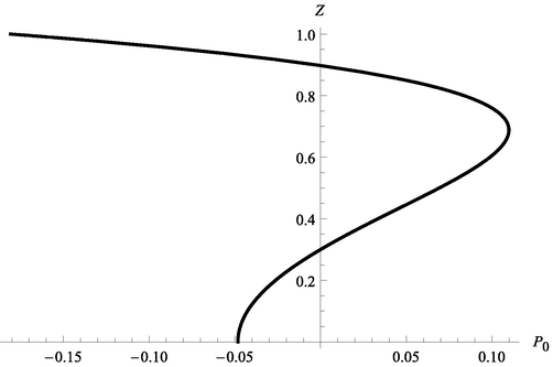

Close

Fig. 7

The profile of the background pressure $P_0$ at $S=1$, ${\psi }_5=0.0006$, ${\psi }_6=0.386$ (the parameters $S$, ${\psi }_5$, ${\psi }_6$ are the coefficients of the exact solution (8)).

Export to PPT

8 Conclusion

The paper presents a new exact solution to the Oberbeck-Boussinesq equations for describing the steady-state thermal diffusion flow of a binary fluid with allowance for the Soret effect. The hydrodynamic fields of velocities, pressure, temperature and concentration are investigated. It has been shown that, at certain values of the boundary conditions and physical coefficients, there are counterflows in the fluid layer (Figs. 2 and 4).

The structure of the exact solution is such that the components ${\mathrm{\Omega }}_x$ and ${\mathrm{\Omega }}_y$ of the vorticity vector $\mathrm{\Omega }=rot\mathit{V}$, coincide up to a constant factor with the tangential stresses ${\tau }_{\mathit{yz}}$ and ${\tau }_{\mathit{xz}}$, respectively. The tangential stresses can have only one zero point in the layer (Fig. 4). Thus, each of the vorticity vector components can vanish at most once (the vortex in the direction of the x- and y-axes changes its direction). In this case, the tangential stresses in the fluid change from tensile to compressive ones (or vice versa). The study of the exact solution allows us to state that the temperature field and the concentration field can be stratified (take the reference value given at the lower boundary) into two zones. For the pressure field, there may exist three portions across the layer thickness, in which the pressure differs from the reference value (atmospheric pressure).

References

- Properties of solutions for the problem of a joint slow motion of a liquid and a binary mixture in a two-dimensional channel. J. Appl. Ind. Math.. 2018;12:395-408.
- [CrossRef] [Google Scholar]
- On thermocapillary instability of a liquid column with a co-axial gas flow. J. Siberian Federal Univ. Math. Phys.. 2013;6:3-17.
- [Google Scholar]
- On laminar flows of planar free convection. Rus. J. Nonlin. Dyn.. 2013;9:651-657.
- A new class of exact solutions for three-dimensional thermal diffusion equations. Theor. Found. Chem. Eng.. 2016;50:286-293.
- Nonstationary laminar thermal and solutal Marangoni convection of a viscous fluid. Comput. Cont. mech.. 2015;8:445-456.
- Unsteady-state Bénard–Marangoni convection in layered viscous incompressible flows. Theor. Found. Chem. Eng.. 2016;50:132-141.
- Vortical Flows of the Advective Nature in a Rotating Fluid Layer. Perm: Perm State Univ. Publ; 2006.
- An Introduction to Fluid Dynamics. Cambridge: Cambridge University Press; 2000.
- Convective instability of Marangoni-Poiseuille flow under a longitudinal temperature gradient. J. Appl. Mech. Tech. Phys.. 2011;52:74-81.
- Thermocapillary convection in a horizontal layer of liquid. J. Appl. Mech. Tech. Phys.. 1966;7:43-44.
- The development of Marangoni convection induced by local addition of a surfactant. Fluid Dyn.. 2011;46:890-900.
- A large-scale layered stationary convection of an incompressible viscous fluid under the action of shear stresses at the upper boundary. Velocity field investigation. Vestn. Samar. Gos. Tekh. Univ. Ser. Fiz.-Mat. Nauki.. 2017;21:180-196.
- Exact solutions for natural convection of layered flows of a viscous incompressible fluid with specified tangential forces and the linear distribution of temperature on the layer boundaries. DReaM. 2017;4:16-31.
- A large-scale layered stationary convection of a incompressible viscous fluid under the action of shear stresses at the upper boundary. Temperature and pressure field investigation. Vestn. Samar. Gos. Tekh. Univ. Ser. Fiz.-Mat. Nauki.. 2017;21:736-751.
- Nonequilibrium Thermodynamics: Transport and Rate Processes in Physical, Chemical and Biological Systems (second ed.). Amsterdam: Elsevier; 2007.
- Ueber die Diffusion der Gase durch poröse Wände und die sie begleitenden Temperaturveränderungen. Arc. Phys. Nat. Sci. Geneve.. 1872;45:490-492.
- On the influence of the Earth’s rotation on ocean-currents. Ark. Mat. Astron. Phys.. 1905;2:1-52.
- Double-diffusive Salt Finger Convection in a Laminar Shear Flow. Saarbrucken: LAP Lambert Academic Publishing; 2011.
- Controlling Marangoni-induced instabilities in spin-cast polymer films: How to prepare uniform films. Eur. Phys. J. E. 2016;39:90.
- Convective Stability of Incompressible Fluids. Jerusalem: Keter Publishing House; 1976.
- Interpretation of the unusual fluid distribution in the Yufutsu gas-condensate field. SPE J.. 2003;8:114-123.
- Dip coating in the presence of an opposing Marangoni stress. Eur. Phys. J. E. 2017;40:9.
- Solutal Marangoni flows of miscible liquids drive transport without surface contamination. Nat. Phys.. 2017;13:1105-1110.
- Simulation of turbulent flow around a tear-shaped body with a tapered flare. Tech. Phys. The Rus. J. Appl. Phys.. 2007;52:991-997.
- Dynamic properties of molecularly thin liquid films. Science. 1988;240:189-191.
- Two-dimensional flows of a viscous binary fluid between moving solid boundaries. J. Appl. Mech. and Tech. Phys.. 2011;52:212-217.
- Sull espansione delle goccie di un liquido galleggiante sulla superficie di altro liquid. Pavia: Tipografia dei fratelli Fusi; 1865.
- Impact of an insoluble surfactant on the thresholds of evaporative Bénard-Marangoni instability under air. Eur. Phys. J. E. 2017;40:90.
- Shear Flow Over Smooth and Wavy Interfaces. Saarbrucken: LAP Lambert Academic Publishing; 2010.
- Viscous near-wall flow in a wake of circular cylinder at moderate Reynolds numbers. Thermophys. Aeromech.. 2017;24:873-882.
- Hydrodynamic Fluctuations in Fluids and Fluid Mixtures. Amsterdam: Elsevier; 2006.
- Free Convection Under the Condition of the Internal Problem. Washington: National Advisory Committee for Aeronautics; 1958.
- New class of exact solutions for Navier-Stokes equations with power dependence of velocities on two spatial coordinates. Theor. Found. Chem. Eng.. 2019;53:112-120.
- On double diffusive convection with Soret effect in a vertical layer between co-axial cylinders. Physica D: Nonlin. Phen.. 2006;215:191-200.
- On the cross-diffusion and Soret effect in multicomponent mixtures. Micrograv. Sci. Tech.. 2009;21:37-40.
- Three-dimensional instability of flow in a flat channel between elastic plates. Comp. Math. Math. Phys.. 2012;52:1445-1451.
- Stability and Transition in Shear Flows (Applied Mathematical Sciences Vol. 142). New York: Springer-Verlag; 2001.
- Plane-parallel advective flow in a horizontal incompressible fluid layer with rigid boundaries. Fluid Dyn.. 2014;49:438-442.
- Sur l'́etat d'équilibre que prend au point de vue de sa concentration une dissolution saline primitivement homohéne dont deux parties sont portées a des températures différentes. Arch. Sci. Phys. Nat.. 1879;2:48-61.
- Complex bifurcations in Benard-Marangoni convection. J. Phys. A: Math. Theor.. 2016;49:e424001