

Translate this page into:
On existence of certain delta fractional difference models
⁎Corresponding author. pshtiwansangawi@gmail.com (Pshtiwan Othman Mohammed),
-
Received: ,
Accepted: ,
This article was originally published by Elsevier and was migrated to Scientific Scholar after the change of Publisher.
Abstract
The discretization of initial and boundary value problems and their existence behaviors are of great significance in various fields. This paper explores the existence of a class of self-adjoint delta fractional difference equations. The study begins by demonstrating the uniqueness of an initial value problem of delta Riemann–Liouville fractional operator type. Based on this result, the uniqueness of the self-adjoint equation will be examined and determined. Next, we define the Cauchy function based on the delta Riemann–Liouville fractional differences. Accordingly, the solution of the self-adjoint equation will be investigated according to the delta Cauchy function. Furthermore, the research investigates the uniqueness of the self-adjoint equation including the component of Green’s functions of and examines how this equation has only a trivial solution. To validate the theoretical analysis, specific examples are conducted to support and verify our results
Keywords
26A48
26A51
33B10
39A12
39B62
Riemann–Liouville operator
Self-adjoint equation
Green’s functions
Existence and uniqueness

Data availability
No data was used for the research described in the article.
1 Introduction
One of the common areas of applied and pure mathematics is discrete fractional calculus with many applications, which deals with non-integer sums and differences. It has been viewed for a very long time as a purely theoretically interesting subject but later, several applications in engineering and physics modeled by discrete fractional calculus. Discrete fractional calculus has become a discretization field of fractional calculus that supported by computational and sum representations; see e.g. Goodrich and Peterson (2015), Wu and Baleanu (2015) and Mozyrska et al. (2019).
Discrete fractional analyses are always positioned to work on common models of applied and pure mathematics due to their unique potentials to identify memory effects. These are related to real-world applications and included theories regarding signal processing, dynamical system, chaos, financial perspectives, impulsive perturbations, and further different aspects; see e.g. Ostalczyk (2015) and Atici et al. (2017).
Recent literature explores diverse computational methodologies for fractional boundary and initial value models across different physical domains. Also, with the development of discrete fractional operators and the discrete fractional analysis, the extension of discrete initial value problems (see e.g. Goodrich (2012), Wang et al. (2020b), Ahrendt et al. (2012)) and boundary value problems of fractional difference models have brought great convenience to researchers (see e.g. Wang et al. (2020a), Almusawa and Mohammed (2023), Baleanu et al. (2023), Chen et al. (2019)). For a discrete system, the initial value problem (IVP) and boundary value problem (BVP) of a fractional difference equation (FDE) model can be regarded as the problem of finding the stability analysis of the discrete system when the initial time conditions and the function in the right sides are known. Evidently, the stability analysis, existence and uniqueness of the solution to the IVP of fractional difference types are important when analyzing fractional difference equations; see e.g. Mohammed and Abdeljawad (2020), Brackins (2014) and Gholami and Ghanbari (2016). Furthermore, different fractional and discrete fractional self-adjoint models, and Green’s function for boundary value problems involving fractional difference models are analyzed by the scholars which are available in the literature as Brackins (2014), Kilbas et al. (2006), Cabada et al. (2021) and Ahrendt and Kissler (2019).
In this paper, we first apply existence and uniqueness theorem of the fractional IVP (in Lemma 2.1) to show the uniqueness and regularity of the other results. Using the variation of constants formula, we will continue to introduce a Cauchy function an solve the self-adjoint problem. In addition, our focus is in fact mainly on the Green’s function in the sense of discrete fractional operators and novel Cauchy functions.
The rest of the paper is structured as follows: The literature of delta fractional operators has been reviewed in Section 2, and then an essential lemma has been stated and proved. Section 3 is reserved for a presentation of main results regarding fractional self-adjoint problems. In Section 4, the Cauchy function considering the falling function is defined. Then, in the same section, we analyze the self-adjoint problem to get the uniqueness and triviality of the function. Finally, in Section 5, we summarize the content of the paper.
2 Preliminaries
Let
,
and
, for
, where
represents the natural numbers. Further, let
such that
, for some
. Then, it is defined in Goodrich and Peterson (2015, Definition 2.25) the
fractional sum operator as follows:
A major property of the composition of delta fractional sum and difference is proved in Abdeljawad (2018), which is given by
Definition 2.1 see Brackins (2014)
For the homogeneous FDE
we say
, where
, as a Cauchy function such that
is the unique solution of
Here, we will state and prove our main Lemma that will be an essential tool for the next results.
Let
,
, and
be defined on
. Then the fractional IVP
By taking
on both sides of (2.7), we have
Computing the left side of (2.8), we see that
Next, by computing the right side of (2.8), we have
3 Discrete self-adjoint problems
In this section, we examine the existence and uniqueness of the delta fractional self-adjoint IVP.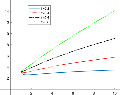
Graph of the function outcome for some values of
.
Let
,
, and
. Then, the fractional IVP
Rewriting (3.1) by using (2.2), we have
We are continuing by using induction and we have to demonstrate that is uniquely determined on . For this, let be the unique solution to (3.1), for and . Then, we have to prove that is also the unique solution of (3.1).
To do this, we use in (3.2), we get This can be solved for , Thus, by considering the hypothesis, each , for in , are known. Therefore, we can say that is also the unique solution of (3.1). Consequently, is the unique solution of (3.1) on . This give us our proof. □
Next, we consider the fractional self-adjoint IVP:
The solution to (3.3) can be expressed by where is as defined in Definition 2.1.
Assume that
and
is a solution of the fractional IVP (3.3). Therefore,
is a solution of
Moreover, by Lemma 2.1, its solution can be represented as
It can be divided both sides by
to get
By summing both sides
, we have
Let and can satisfy Then, , for .
Let us set , and Therefore, solves the IVP Thus, by using Theorem 3.2, we see that and this implies that . Thus, the proof has been done. □
4 BVPs with Green’s function
This section is dedicated to examine the Green’s function for homogeneous and nonhomogeneous fractional BVPs with homogeneous BCs.
Let
be two real numbers such that
,
, and
. Then, the fractional BVP
Let
, and let
. Then, by using Lemma 2.1, the solution
of the fractional IVP
is given by
By setting
and using
, we have
By summing both sides
we have
We change the order of sums to have
Next, we generalize the above Green’s function theorem to the following fractional self-adjoint BVP:
The fractional self-adjoint BVP (4.5) has only the trivial solution iff
If we consider
, then it follows from Lemma 2.1 that
that is,
Suppose that
be a quantity as in Lemma 4.1. Then the Green’s function for the BVP (4.5) is expressed by
Suppose that
is a solution of the BVP
5 Concluding remarks
To conclude, our study focuses on the existence, uniqueness and trivial solutions in the classes of self-adjoint equations with delta Riemann–Liouville fractional operators. The uniqueness of the initial value problem on delta fractional difference operators is represented by applying delta fractional sum to both sides of the equation and using some discrete delta properties. By applying this uniqueness theorem, we have analyzed and derived the existence and uniqueness of the proposed self-adjoint delta fractional difference equation. In the other part of our study, the Cauchy function based on the delta Riemann–Liouville fractional differences has been introduced and the self-adjoint problem has been solved accordingly. In addition, the uniqueness of the self-adjoint problem including the component of Green’s functions has been determined. Then, we have examined how this problem has only a trivial solution and the condition under which it has only a trivial solution has been found. Throughout the study, we have presented some examples and through these extensive examples, we have validated the theoretical results.
CRediT authorship contribution statement
Pshtiwan Othman Mohammed: Investigation, Methodology, Writing – original draft. Hari Mohan Srivastava: Conceptualization, Investigation, Writing – original draft. Rebwar Salih Muhammad: Conceptualization, Investigation, Visualization, Writing – review & editing. Eman Al-Sarairah: Data curation, Project administration, Validation. Nejmeddine Chorfi: Funding acquisition, Software, Writing – review & editing. Dumitru Baleanu: Funding acquisition, Investigation, Software, Supervision.
Acknowledgments
Researchers Supporting Project number (RSP2024R153), King Saud University , Riyadh, Saudi Arabia.
Declaration of competing interest
The authors declare that they have no known competing financial interests or personal relationships that could have appeared to influence the work reported in this paper.
References
- Different type kernel –fractional differences and their fractional –sums. Chaos Solit. Fract.. 2018;116:146-156.
- [Google Scholar]
- Laplace transforms for the nabla-difference operator and a fractional variation of parameters formula. Commun. Appl. Anal.. 2012;16:317-347.
- [Google Scholar]
- Cameron Green’s function for higher-order boundary value problems involving a nabla Caputo fractional operator. J. Difference Equ. Appl.. 2019;25:788-800.
- [Google Scholar]
- Approximation of sequential fractional systems of Liouville-Caputo type by discrete delta difference operators. Chaos Solitons Fractals. 2023;176:114098
- [Google Scholar]
- A new approach for modeling with discrete fractional equations. Fund. Inform.. 2017;151:313-324.
- [Google Scholar]
- On convexity analysis for discrete delta Riemann–Liouville fractional differences analytically and numerically. J. Inequal. Appl.. 2023;2023:4.
- [Google Scholar]
- Boundary Value Problems of Nabla Fractional Difference Equations. The University of Nebraska-Lincoln; 2014. (Thesis (Ph.D.))
- Non-trivial solutions of non-autonomous nabla fractional difference boundary value problems. Symmetry. 2021;13:1101.
- [Google Scholar]
- Ulam-Hyers stability of Caputo fractional difference equations. Math. Methods Appl. Sci.. 2019;42:7461-7470.
- [Google Scholar]
- Coupled systems of fractional -difference boundary value problems. Differ. Eq. Appl.. 2016;8:459-470.
- [Google Scholar]
- On discrete sequential fractional boundary value problems. J. Math. Anal. Appl.. 2012;385:111-124.
- [Google Scholar]
- Discrete Fractional Calculus. New York: Springer; 2015.
- A relationships between the discrete Riemann–Liouville and Liouville-Caputo fractional differences and their associated convexity results. AIMS Math.. 2022;7:18127-18141.
- [Google Scholar]
- Theory and Applications of Fractional Differential Equations. Amsterdam, The Netherlands: Elsevier B.V.; 2006.
- Discrete generalized fractional operators defined using h-discrete Mittag–Leffler kernels and applications to AB fractional difference systems. Math. Methods Appl. Sci.. 2020;46:7688-7713.
- [Google Scholar]
- Solutions of systems with the Caputo–Fabrizio fractional delta derivative on time scales. Nonlinear Anal. Hybrid Syst.. 2019;32:168-176.
- [Google Scholar]
- Discrete Fractional Calculus: Applications in Control and Image Processing. World scientific; 2015.
- Discrete fractional Bihari inequality and uniqueness theorem of solutions of nabla fractional difference equations with non-Lipschitz nonlinearities. Appl. Math. Comput.. 2020;367:125118
- [Google Scholar]
- Discrete fractional watermark technique. Front. Inf. Technol. Electron. Eng.. 2020;21:880-883.
- [Google Scholar]
- Discrete chaos in fractional delayed logistic maps. Nonlinear Dynam.. 2015;80:1697-1703.
- [Google Scholar]


