

Translate this page into:
On a new type of non-stationary helical flows for incompressible 3D Navier-Stokes equations
⁎Corresponding author. sergej-ershkov@yandex.ru (Sergey V. Ershkov),
-
Received: ,
Accepted: ,
This article was originally published by Elsevier and was migrated to Scientific Scholar after the change of Publisher.
Peer review under responsibility of King Saud University.
Abstract
In fluid mechanics, a lot of authors have been executing their researches to obtain the analytical solutions of Navier-Stokes equations. But there is an essential deficiency of non-stationary solutions indeed.
In our presentation, we proceed exploring the case of non-stationary helical flows of the Navier-Stokes equations for incompressible fluids, with variable (spatially dependent) coefficient of proportionality α between velocity and the curl field of flow.
The main motivation of the current research is the exploring the case when velocity field u is supposed to be perpendicular to the vector ∇α. Conditions for the existence of the exact solution for the aforementioned type of flows are obtained, for which non-stationary helical flow with invariant Bernoulli-function is considered.
The spatial part of the pressure field of the fluid flow should be determined via Bernoulli-function, if components of the velocity of the flow are already obtained.
Keywords
Navier-Stokes equations
Non-stationary helical flow
Arnold-Beltrami-Childress (ABC) flow

1 Introduction, the Navier-Stokes system of equations
In accordance with (Ladyzhenskaya, 1969; Landau and Lifshitz, 1987), the Navier-Stokes system of equations for incompressible flow of Newtonian fluids should be presented in the Cartesian coordinates as below (under the proper initial conditions):
Besides, we assume here external force F above to be the force, which has a potential ϕ represented by F = −∇ ϕ. As for the domain in which the flow occurs and the boundary conditions, let us consider only the Cauchy problem in the whole space.
Let us search for solutions of the system (1) and (2) in a form of helical or Beltrami flow below:
2 The originating system of PDE for helical non-stationary flow
Using the identity (u⋅∇)u = (1/2)∇(u2) – u × (∇ × u), we could present the Navier-Stokes Eqs. (1) and (2) for incompressible viscous flow u = {u1, u2, u3} as below (Saffman, 1995; Milne-Thomson, 1950):
The continuity Eq. (1) let us obtain as below, using (3):
Let us note that the obvious case ∇α = 0 in (5) was explored properly in (Ershkov, 2016); so, the main motivation of the current research is the obtaining a new solution: we wish to explore the case when velocity field u is to be perpendicular to the vector ∇α - such the idea belongs to Dr. G.B. Sizykh, MIPT, (personal communications).
3 The presentation of time-dependent solutions
Using Eqs. (1) and (3), each equations of the 2-nd vector equation of system (4) could be transformed as below
So, we obtain from (7):
Three aforementioned equations of the system (8) with the additional Eq. (6) should determine 3 time-dependent functions {u1, u2, u3} with additional unknown time-dependent Bernoulli-function B in regard to the time-parameter t.
Using (5), let us obtain the dot product of the components of vector Eq. (7) on components of vector ∇α as below:
Let us search for solutions {u, p} of the system of Eqs. (1) + (7) which should conserve the Bernoulli-function to be the invariant of the aforementioned system:
4 Solving ODE system for time-dependent components of velocity field
Taking into account the basic assumption (11), system of Eq. (7) should be transformed accordingly:
Let us multiply the 1-st equation of system (12) on U, the 2-nd Eq. on V, 3-rd on W
then if we sum all the resulting equations of the system above, we should obtain the proper 1-st integral (invariant) of the system (12):
For the further solving of the system (12), we could use invariants (6) and (13); let us consider, for example, the 1-st equation of system (12):
If we choose ∂α/∂y = 0, then we should obtain from (6) and (13) (∂α/∂z ≠ 0):
In this case, Eq. (14) should be transformed to the ordinary differential equation of the 1-st order, which describes the dependence of the component of velocity U with respect to the time-parameter t (∂α/∂y = 0):
Besides, Eq. (16) can be presented as below:
The right part of the 1-st of the equalities above is proved to be the proper derivative of the right part of the 2-nd equality (Kamke, 1971); it yields the appropriate Abel ordinary differential equation.
We should note that the spatial part of velocity of the flow is determined by the invariant (6), which has been obtained by using of continuity Eq. (1) and the chosen type of helical flow (3). The spatial part of the pressure field of the flow should be determined via Bernoulli-function (11), if components of the velocity of the flow {U, V, W} are already obtained.
5 Final presentation of the solution (the helical flows)
Let us present the non-stationary solution {p, u} of helical flow type (3) for Navier-Stokes Eqs. (1) and (2) in its final form (we consider the case ∂α/∂y = 0):
The dependence of the component of velocity U with respect to the time-parameter t (∂α/∂y = 0) is described by the expression (19) below via parameter λ(t), which is the solution of the Abel ordinary differential equation of the 1-st order (20) with respect to the time-parameter t, as shown below:
6 Discussion
The system of Navier-Stokes equations has already been investigated in many researches including its numerical and analytical solutions (Drazin and Riley, 2006), even for 3D case of compressible gas flow (Ershkov and Schennikov, 2001) or for 3D case of non-stationary flow of incompressible fluid. However essential deficiency exists in the studies of non-stationary solutions of the Navier-Stokes equations.
We have explored here the case of non-stationary flows of helical type for the incompressible Navier-Stokes equations with constant Bernoulli-function (11) in the whole space (the Cauchy problem). In this respect we should refer also to the modern researches (Ershkov, 2015a,b, 2016a,b, 2020) (with the proper examples of non-stationary solutions of Navier-Stokes equations in case of constant Bernoulli-function) or, for example, we should recall the results of comprehensive article (Stepanyants, 2015) (which reports the alternative example of using the Bernoulli-invariant to obtain analytical non-stationary solutions of the Navier-Stokes system of equations). Also it would be useful for common readers if we put explicitly why we consider a case where Bernoulli function is constant (according to the suggestion of esteemed Reviewer): let us opt to add an Appendix to demonstrate that this is the case, see for example (https://math.stackexchange.com/questions/1641862/prove-bernoulli-function-is-constant-on-streamline).
In addition to the results of aforementioned articles (Ershkov, 2015a,b, 2016a,b, 2020), we have obtained in this derivation the analytical non-stationary helical solutions of the Navier-Stokes equations for incompressible fluids, which should conserve the Bernoulli-function for the flow; namely, in this paper we have explored the case when velocity field u is perpendicular to the vector ∇α (5) for incompressible fluids by extending the case of constant α to the case (3) where α depends on variables (x,y,z).
We have proved that the aforementioned solution exists, when appropriate initial and boundary conditions are provided. Moreover, we suggest the appropriate form of the exact solution in case of the constant Bernoulli-function (11).
According to our understanding, we could use such the mathematical results as tools (for applying them to clarify the ambiguity in open problem which takes place in fluid mechanics) and we need to discuss accordingly such the application of results as below.
So, the aforementioned open problem could be formulated as follows: a well-known statement exists that solutions of the Navier-Stokes momentum Eq. (2) (along with the continuity Eq. (1)) could be obtained from solutions of the reduced curl-version of Navier-Stokes momentum Eq. (2); moreover, one of the authors (Sergey Ershkov) met specialists in fluid mechanics (Prof. V.Zhmur, MIPT, personal communications) who assumed that if we take the curl from both the sides of Navier-Stokes momentum Eq. (2), we should obtain the equation which is equivalent to the Navier-Stokes momentum Eq. (2) (in the sense of existence of solutions). This is obviously wrong point of view which reduces variety of the solutions of the Navier-Stokes momentum Eq. (2) to only the curl solutions (excepting the irrotational or curl-free part of velocity field). Let us recall that, in accordance to the Helmholtz fundamental theorem of vector calculus, velocity field is proved to be presented as the sum of irrotational (curl-free) part of the field of flow velocity along with solenoidal (divergence-free) part of the field of flow velocity.
Let us prove by using the properties of the new type of helical flows, which has been constructed in the current research, the suggestion above about the equivalence of the Navier-Stokes momentum Eq. (2) to its reduced curl-version is not correct.
For the obtaining of the curl-version of the Navier-Stokes momentum Eq. (2), we need take the curl from both the sides of Navier-Stokes momentum Eq. (2). Let us consider non-stationary helical flows (3), for which the Navier-Stokes momentum Eq. (2) is proved to be simplified accordingly (see (7)):
Let us transform Eq. (7), by using of helical flow assumption (3) as below:
As we can see from Eq. (21), it describes the correct dynamics of the curl field Ω, which has been obtained from the Navier-Stokes momentum Eq. (2) by the equivalent transformations. But it obviously differs from the case if we simply take the curl from both the sides of the Eq. (7), indeed:
For the helical flow with constant coefficient α = const, Eq. (21) could be reduced as below:
Where the last equation above states the strong link between spatial parts of the pressure field, the curl field Ω and coefficient α (x, y, z). In case of variable coefficient α (x, y, z), the term ∇α × Ω ≠ 0 is the essential difference with respect to Eq. (21).
As for the relevance of this new solution, let us discuss the essential details about the possible physical properties of the aforementioned solution (18)–(20).
Eq. (20) is known to be an Abel ODE of the second kind, a kind of generalization of the Riccati ODE. We also note that due to the special character of the solutions of Riccati-type ODEs (Kamke, 1971), there is the possibility for sudden jumping in the magnitude of the solution at some time t₀ (Ershkov, 2017a, b, c) (with restriction on function U(t), which is given in (15)).
In the physical sense, such the aforementioned jumping of Riccati-type solutions of Eq. (20) could be associated with the effect of a sudden acceleration/deceleration of the flow velocity (the component U(t)) at a definite moment of parametric time t₀. This means that there exists a potential for a kind of gradient catastrophe (Arnold, 1992), depending on the initial conditions.
We have schematically imagined the Riccati-type solution (Ershkov, 2016) of equations of a type (20) at Fig. 1 below which demonstrates the possibility for sudden jumping in the magnitude of the solution at some time t₀.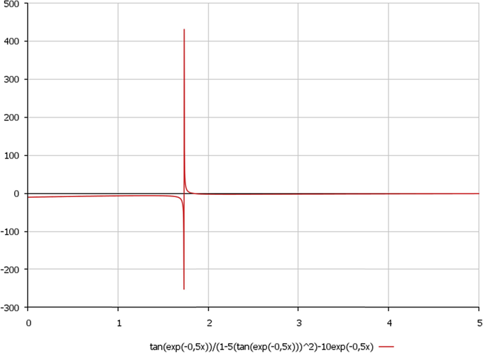
Schematically presented the Riccati-type solution of a type (20) (Ershkov, 2016), here we designate x = t just for the aim of presenting the plot of solution.
Mathematical procedure for reduction of the solution of a type (20) to the appropriate simplifyed Riccati-type solution has been moved to an Appendix.
7 Conclusion
The main motivation of the current research is the developing of the investigation of the case of non-stationary helical flows for incompressible Newtonian fluids, the 1st type of which (α = const) was successfully investigated in (Ershkov, 2016).
While such a theoretical motivation is of course understood, let us also add that helical flows is very important in some practical problems, for example in wind turbine design etc.
Therefore, we should especially emphasize regarding the significance of the aforementioned helical flows of 3D Navier-Stokes equations: both theoretical motivation, and also practical motivation. Indeed, helical flows are often found in the real engineering problems of flows, which concern the fast rotating of coaxial propellers or air-screws of various types of aircrafts. This is a sound and useful applications of hydrodynamics theory, which illuminate the fact of successive implementation of theoretical developments in a real design of our life as modern reality.
We begin from form of helical flows (3), distinguished by spatial dependence of the coefficient of proportionality α (x, y, z) between velocity and curl field of fluid flow.
The using such the spatially dependent coefficient in analysis of the continuity Eq. (1) yields Eqs. (5) and (6). We should also note that obvious case α = const in (5) was explored earlier in (Ershkov, 2016); so, the main motivation of the current research is the exploring the case when velocity field u is to be perpendicular to the vector ∇α – such the idea belongs to Dr. G.B.Sizykh, MIPT (personal communications).
Then we have obtained conditions (9), (10) to be valid from the analysis of momentum Eq. (2) in a form (7), (8), which means that gradient of the Bernoulli function ∇B should also be perpendicular to the vector ∇α.
We assume for solutions {u, p} of the system of Eqs. (1) + (7) that Bernoulli-function (11) should be invariant for the aforementioned system. Such an assumption simplifies momentum equation to the form (12), from which we obtain a first integral (invariant) (13). For further solving of the system (12), we could use invariants (6) and (13); then let us consider, for example, the 1-st equation of (12) in a form (14).
For the partial case ∂α/∂y = 0, system (14) could be reduced via presentation of the components V, W (15) to the ordinary differential equation of the 1-st order (16).
We should note that the spatial part of velocity of the flow is determined by the invariant (6), which has been obtained by using of continuity Eq. (1) and the chosen type of helical flows (3). The spatial part of the pressure field of the fluid flow should be determined via Bernoulli-function (11), if components of the velocity of the flow {U, V, W} are already obtained (which are determining via the choosing of the special form of variable coefficient α (x, y, z)).
Also we should note that since the fluid is incompressible for the development above, there is a strong link between initial conditions and the solution inside.
Besides, final presentation of the components of velocity field as well as pressure field is valid only under special conditions, which restrict the choosing of the form of variable coefficient α (x, y, z).
As we know, ABC-ansatz (Ershkov, 2016; Arnold, 1965; Dombre, 1986) was published as a solution of the steady problem. In their work, they never realized that its extension is possible also to the non-stationary problem. It was extended for the first time in 1919 in (Trkal, 1994) to the non-stationary problem as a time-kinematic viscosity decaying solution; also we should mention the comprehensive article (Bogoyavlenskij and Fuchssteiner, 2005) in regard to the non-stationary helical flows with the special kind of the spatial part for the velocity fields as well as the appropriate pressure gradient field.
It should be additionally noted that some mathematical solutions don't reflect physical phenomena and the equation for the force, F, used in the analysis, is valid only for conservative forces (Ershkov, 2015). The assumption that the body force F is conservative means its curl is zero which means it is incapable of generating any vorticity. But vorticity, associated with the curl field, is assumed to be arising due to the proper sources of vorticity in the flow of fluids (Ershkov, 2016). For example, such the sources could be associated with the solid surface or pressure gradient, influence of viscous forces, Coriolis forces or the curving shock fronts when speed is supersonic.
The stability of the presented solution is not considered. In this respect we confine ourselves to mention the paper (Podvigina and Pouquet, 1994), in which all the difficulties concerning the stability of the close-related ABC-flows are remarked. In (Podvigina and Pouquet, 1994) the nonlinear regime was successfully investigated by Podvigina and Pouquet, who found complicated switching between nonlinear time-dependent ABC states.
The last but not least, we should especially mention the comprehensive modern researches (Moffat, 2014; Changchun, 1991; Savas Can Selçuk, 2016), where a lot of unknown details concerning the close-related area of helical flows are remarked.
Conflict of interest
Authors declare that there is no conflict of interests regarding publication of article.
Remark regarding contributions of authors as below:
In this research, Dr. Roman Shamin (PhD-tutor of Sergey V. Ershkov) performed the general scientific management of the direction of creative scientific search. Sergey Ershkov is responsible for the results of the article, the obtaining of exact solutions, simple algebra manipulations, calculations, the representation of a general ansatz and calculations of graphical solutions, approximation and also is responsible for the search of approximate solutions. Ayrat Giniyatullin is responsible for the plots and graphical solutions.
Acknowledgements
Authors are thankful to Dr. G.B.Sizykh (Golubkin and Sizykh, 1987), Dr. A.V.Koptev (Koptev, 2014), Dr. V.I.Semenov (Semenov, 2014), and especially to Dr. G.V.Alekseev (Alekseev, 2016) with respect to the fruitful discussions during preparing of this manuscript.
This study was initiated in the framework of the state task programme in the sphere of scientific activity of the Ministry of Education and Science of Russian Federation (project No. 5.5176.2017/8.9) and was performed with the financial support of the grants of the President of the Russian Federation for state support of leading scientific schools of the Russian Federation (NSH-2685.2018.5) and young Russian scientists - candidates of science (MK-1124.2018.5).
References
- Solvability of an inhomogeneous boundary value problem for the stationary magnetohydrodynamic equations for a viscous incompressible fluid. Differential Eqs.. 2016;52(6):739-748.
- [Google Scholar]
- Sur la topologie des 'ecoulements stationnaires des fluids parfaits. CR Acad. Sci. Paris. 1965;261:17-20.
- [Google Scholar]
- Catastrophe Theory, 3-rd Ed. Berlin: Springer-Verlag; 1992.
- Exact NSE solutions with crystallo-graphic symmetries and no transfer of energy through the spectrum. J. Geometry Phys.. 2005;54(3):324-338.
- [Google Scholar]
- Some properties of three-dimensional Beltrami flows. ACTA Mechanica Sinica. 1991;7(4):289-294.
- [Google Scholar]
- The Navier-Stokes Equations: A Classification of Flows and Exact Solutions. Cambridge: Cambridge University Press; 2006.
- Quasi-periodic solutions of Einstein-Friedman equations. Int. J. Pure Appl. Math.. 2014;90(4):465-469.
- [Google Scholar]
- New exact solution of Euler’s equations (rigid body dynamics) in the case of rotation over the fixed point. Arch. Appl. Mechan.. 2014;84(3):385-389.
- [Google Scholar]
- On existence of general solution of the Navier-Stokes equations for 3D non-stationary incompressible flow. Int. J. Fluid Mech. Res.. 2015;42(3):206-213. Begell House
- [Google Scholar]
- Quasi-periodic non-stationary solutions of 3D Euler equations for incompressible flow. J. King Saud Univ. – Sci.. 2015;27:369-374.
- [Google Scholar]
- Non-stationary helical flows for incompressible 3D Navier-Stokes equations. Appl. Math. Comput.. 2016;274:611-614.
- [Google Scholar]
- About existence of stationary points for the Arnold-Beltrami-Childress (ABC) flow. Appl. Math. Comput.. 2016;276:379-383.
- [Google Scholar]
- A procedure for the construction of non-stationary Riccati-type flows for incompressible 3D Navier-Stokes equations. Rendiconti del Circolo Matematico di Palermo. 2016;65(1):73-85.
- [Google Scholar]
- Non-stationary Riccati-type flows for incompressible 3D Navier-Stokes equations. Comput. Math. Appl.. 2016;71(7):1392-1404.
- [Google Scholar]
- Revolving scheme for solving a cascade of Abel equations in dynamics of planar satellite rotation. Theoret. Appl. Mechan. Lett.. 2017;7(3):175-178.
- [Google Scholar]
- A Riccati-type solution of Euler-Poisson equations of rigid body rotation over the fixed point. Acta Mechan.. 2017;228(7):2719-2723.
- [Google Scholar]
- Forbidden zones for circular regular orbits of the moons in solar system, R3BP. J. Astrophy. Astron.. 2017;38(1):1-4.
- [Google Scholar]
- A Riccati-type solution of 3D Euler equations for incompressible flow. J. King Saud Univ. – Sci.. 2020;32:125-130. https://www.sciencedirect.com/science/article/pii/S1018364718302349
- [Google Scholar]
- Self-similar solutions to the complete system of navier-stokes equations for axially symmetric swirling viscous compressible gas flow. Comput. Math. Math. Phys. J.. 2001;41(7):1117-1124.
- [Google Scholar]
- https://math.stackexchange.com/questions/1641862/prove-bernoulli-function-is-constant-on-streamline.
- Hand-Book for Ordinary Differential Eq.. Moscow: Science; 1971.
- Generator of solutions for 2D Navier - Stokes equations. J. Siberian Federal Univ. Math. Phys.. 2014;7(3):324-330.
- [Google Scholar]
- The Mathematical Theory of viscous Incompressible Flow (2nd ed.). New York: Gordon and Breach; 1969.
- Fluid mechanics, Course of Theoretical Physics 6 ((2nd revised ed.)). Pergamon Press; 1987. ISBN 0-08-033932-8
- Theoretical Hydrodynamics. Macmillan; 1950.
- Vortex Dynamics. Cambridge University Press, ISBN; 1995. 0-521-42058-X
- Savas Can Selçuk (2016), Numerical study of helical vortices and their instabilities, Mechanics of the fluids [physics.class-ph]. Université Pierre et Marie Curie - Paris VI, 2016. English. <NNT: 2016PA066138>. PhD-thesis, 200 pages.
- Some new identities for solenoidal fields and applications. Mathematics. 2014;2:29-36. 3390/math2010029
- [Google Scholar]
- The bernoulli integral for a certain class of non-stationary viscous vortical flows of incompressible fluid. Stud. Appl. Math.. 2015;135:295-309. Wiley Periodicals, Inc., DOI: 10.1111/sapm.12087
- [Google Scholar]
- A note on the hydrodynamics of viscous fluids (translated by I. Gregora) Czech. J. Phys.. 1994;44:97-106.
- [Google Scholar]
Appendix
Eq. (20) is known to be an Abel ODE of the second kind (Kamke, 1971), a kind of generalization of the Riccati ODE. Moreover, one can obviously reduce (or simplify) this type of equation to the Riccati type of ODE, if conditions below for the coefficients {f, g, h} in (17) via appropriate coefficients in (20) are valid (for all variety of λ(t), at any moment of time t):
where I = (1 second)2; F₇, F₈ are proper coefficients which to be determined as below
Let us simplify conditions (A.1) via the expressions for coefficients {f, g, h} in (17) accordingly:
As we can see from (A.3), each of Eqs. (A.2) and (A.3) has been simplified to only one demand or restriction with respect to the choosing of the form of parameter α (x, y, z):
Thus, Eq. (20) has been reduced via additional assumptions (A.1)–(A.4) from Abel to Riccati type of ODE:
The left side of equation above could be transformed to the proper quadrature (Ershkov, 2015) in regard to parameter λ(t):
Thus, by the proper obtaining of re-inverse dependence of a solution from the time t (Ershkov, 2014b) we could present the expression for parameter λ(t) as below (just for simplicity, let us choose the constants of the solution so that Δ = 2 in (A.6)):
So, we obtain from (19) and (A.7) (see Fig. 2 below):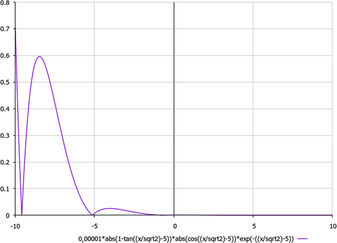
Schematically presented the Riccati-type solution (A.8), here we designate x = t just for the aim of presenting the plot of solution.
The components of the velocity of the flow {V, W} should be determined via formulae (18) (where expression for U is given in (A.8) above), see Fig. 3:
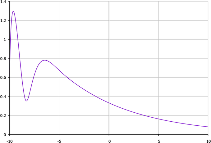
Schematically presented component V of the flow velocity, which corresponds to the simplified case (A.8) of the solution (here we designate x = t just for the aim of presenting the plot of solution).
But the pressure field p should be determined via Bernoulli-function (11) (once components of the velocity of the flow {U, V, W} are calculated), for example as below (see Fig. 4):
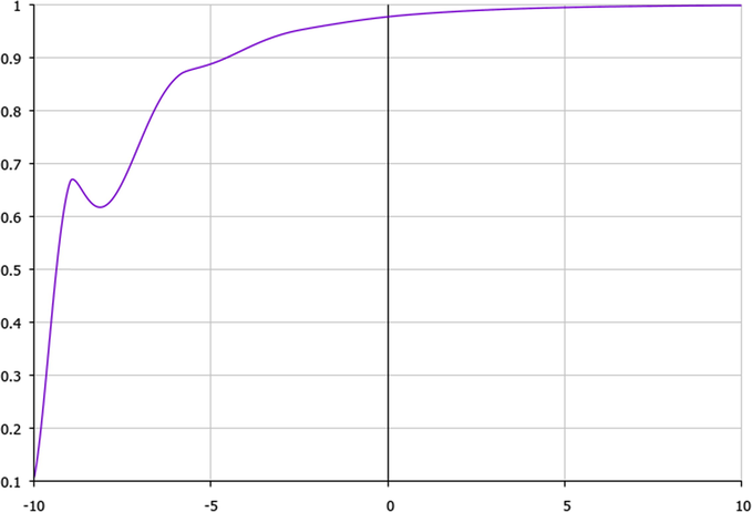
Schematically presented pressure field p of the flow, which corresponds to the simplified case (A.8) of the solution (here we designate x = t just for the aim of presenting the plot of solution).


