Numerical study of the solitary wave shoaling phenomena using KdV Equation

1 Introduction

As a non-breaking wave propagates from an area of great depth to shallow water, the conservation of wave energy flux leads to an increase in wave amplitude and a decrease in wavelength. This phenomenon is known as shoaling. Waves that begin to shoal closer to the shore, like regular surf waves, undergo relatively small changes in crest height. In contrast, tsunami waves, which undergo shoaling farther away from the coast, have their heights greatly amplified by this process. Tsunami waves with amplitudes of less than one meter in deep water can reach heights of fifteen to thirty meters by the time they reach the shore (Tsunami shoaling, 2011).

The destructive effect of shoaling is well-documented. The WHO estimates that, between 1998 and 2017, at least 250 thousand deaths were caused by tsunamis (Tsunamis, 2021). In terms of material losses, a press release (UNDRR, 2018) from the United Nations Office for Disaster Risk Reduction cited that US$280 billion in damages were incurred by tsunamis within the same twenty-year period. The destructive factors that make tsunamis so devastating also occur in smaller cases of shoaling-related disasters. Tall waves damage man-made structures and sweep debris into human-populated areas, causing injuries and death. Inhabitants of coastal communities, who rely on the ocean for their livelihoods, often drown when high waves inundate the coast. Thus, due to its ability to transform harmless-seeming waves into extremely effective agents of destruction, shoaling has long captured the interest of researchers and engineers.

As a result, many studies have been conducted on the effects, causes, and characteristics of shoaling. Research on shoaling tends to focus on non-solitary waves, as investigating solitary waves tend to require solving equations with complicated boundary conditions. Coupled equations, such as Boussinesq-type equations, are often used to describe the motion of these waves. Analytical (Madsen and Sørensen, 1992; Simarro et al., 2013) and numerical (Galan et al., 2012; Ozanne et al., 2000; Ghadimi et al., 2012; Nwogu, 1993; Madsen et al., 2002; Do Carmo et al., 1993; Beji and Nadaoka, 1996; Grilli et al., 1994; Zhao et al., 2004) solutions to these equations were able to shed light on how non-solitary waves behave when they undergo shoaling over uneven bottom. Models based on the Reynolds Averaged Navier Stokes equations have also been used to carry out numerical studies of wave shoaling (Eldrup and Lykke Andersen, 2020; Srineash and Murali, 2018). Magdalena and Iryanto (2018) solved the Shallow Water Equations analytically and numerically in order to model the effects of wave shoaling. In our previous study, only linear waves are considered. A single, uncoupled equation from the Korteweg-de Vries (KdV) family is able to describe the movement of a solitary wave as it undergoes shoaling while taking into account non-linear and dispersive effects. Thus, a KdV-type equation is used to tackle this problem. The KdV-type equation has been used to explain several wave problems (Mouassom et al., 2021; Fokou et al., 2016). The higher-order terms in the KdV-type equation make it relatively difficult to solve both numerically and analytically, though most studies opt to narrow down the problem to a specific set of cases so that analytical solutions can be obtained. However, these analytical solutions are not general and must be re-derived for different situations. Numerical methods, on the other hand, can be generalized and applied to a wide variety of cases. The numerical methods for solving KdV-type equations tend to use second-order finite difference methods, resulting in noticeable dispersion errors.

A higher-order finite difference method, which is the fourth-order finite difference method, has been used previously by Wang and Dai (2019) to solve the KdV-type equation numerically. In this case, the governing equation used is the generalized Rosenau-KdV equation. However, Wang and Dai (2019) used the 4th-order finite difference method to approximate only the higher spatial derivative terms in the equation ( $u_{\mathit{xxx}}$ ). In addition, the study was conducted to describe wave problem in a flat bottom condition, so wave shoaling phenomena was not considered. Therefore, in this research, we propose a modified fourth-order finite difference method, where we consider the bottom of the water channel to be uneven which results in the occurrence of wave shoaling phenomena. In order to simulate wave shoaling over an uneven bottom topography correctly, a certain adjustment is needed when implementing the 4th-order finite difference method into the KdV-type equation, especially for the last term in the equation. In this case, we also apply the 4th-order finite difference method to all of the spatial derivative terms in the equation, instead of the higher ones only. The results obtained using this method are compared to analytical results obtained by Karczewska and Rozmej (2020), which presented the derivation of KdV-type equations for solitary waves propagating in shallow areas with uneven bottoms. Our method reduces the dispersion error considerably and produces results that are remarkably similar to the analytical solutions provided by Karczewska and Rozmej (2020).

The cases investigated in this paper involve the parameters $\alpha$ and $\beta$ , which affect the velocity potential of the wave. Numerical simulations are run for $\beta =O(\beta )$ , with two values of $\alpha$ , which are $O(\beta )$ and $O({\beta }^2)$ . Simulation results are used to analyze each factor and draw conclusions regarding how they affect the behavior of waves undergoing shoaling.

This paper is organized as follows. In Section 2, the governing equations are discussed. Section 3 presents the derivation of the analytical solutions, and the numerical method is explained in Section 4. The results of the simulations are presented and analyzed in Section 5. Section 6 concludes the paper with a summary of the results and recommendations based on the results.

2 Mathematical model

This section discusses the KdV-type equation that will be used to simulate wave propagation over an uneven bottom topography. Karczewska and Rozmej (2020) developed several variations of the KdV-type equation. However, in this research, we will focus on wave propagation across an uneven bottom by employing the first-order KdV-type equation. In this situation, we configure the model as shown in Fig. 1. A wave of amplitude a, wavelength L, and surface elevation $\eta (x,t)$ propagates along a water channel with an irregular bottom topography of $h(x)$ . The water channel has a maximum undisturbed depth of H and an amplitude of $a_h$ for the bottom variation.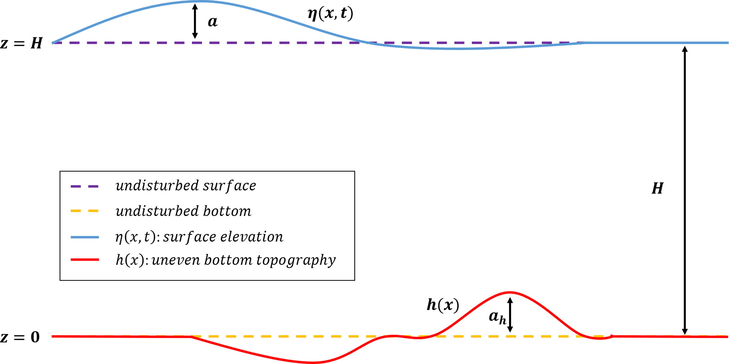

Close

Fig. 1

Illustration of model setup and configuration.

Export to PPT

Now, in deriving a shallow water model, it is a common approach to assume that the fluid is inviscid, incompressible, and irrotational. Under that assumption, the velocity potential $\varphi$ will satisfies Laplace equation as well as the boundary conditions corresponding to it. Those equations are

Applying those non-dimensional variables to Eq. (1) and following the steps explained by Karczewska and Rozmej (2020), Karczewska et al. (2014), the KdV-type equation can finally be derived. To make the writing convenient, all the tildes will be ignored from here onward. In addition, small (perturbation) parameters are introduced. Two of them are the common used small parameters which are $\alpha =a/H$ and $\beta ={(H/L)}^2$ . A new small parameter introduced by Karczewska and Rozmej (2020), Karczewska et al. (2014) is $\delta =a_h/H$ . Several cases were studied by Karczewska and Rozmej (2020) for different configuration of the order of the three small parameters. For Case 1 that we will observe here, the configuration is $\alpha =O(\beta )$ and $\delta =O(\beta )$ . According to Karczewska and Rozmej (2020), the first order KdV-type equation of Case 1 can be written as

On a note, this model is only applicable for the case where $h(x)=\mathit{kx}$ , with k is the slope of the topography. Using the model, we will simulate wave propagation over a slope, specifically when wave shoaling phenomenon is generated.

3 Analytical solutions

Here, the analytical solution of Case 1 KdV-type equation over a flat bottom will be briefly explained. The equation that is needed to be solved is Eq. (3). However, since we will only solve the equation for wave propagation over a flat bottom, we fix $\delta =0$ . Hence, the last term in the equation, which is $-\frac{1}{4}\delta (k\eta +2\mathit{kx}{\eta }_x)$ is vanished. Now, consider an assumption where a solitary wave propagates to the right direction with its surface elevation defined as $\eta (x,t)=\eta (x-\mathit{vt})$ . Therefore, we have ${\eta }_t=-v{\eta }_x$ , meaning that Eq. (3) can be rewritten as

In this case, we assume that the solution of the equation is in the form of a soliton with $\eta (x,t)=A{\mathrm{sech}}^2(B(x-\mathit{vt}))$ , in which A is the initial amplitude and v is the wave speed. Using the derivation that is about to be explained, we aim to obtain the unknown parameter B as a function of $\alpha ,\beta$ , and A, which will help us to define v later on. Substitute the above assumption to Eq. (5) yields

4 Numerical scheme

In this section, we will derive a numerical model using the 4th-order forward time centered space. This method improves the wave shape and dissipation error as found when we use the numerical approach provided by Zabusky and Kruskal (1965). In this scenario, we set a numerical domain where $[0,l]$ is the spatial domain and $[0,t]$ is the time domain. The spatial domain is then partitioned into N grids with length of $\mathrm{\Delta }x$ . The time domain is divided into M grids in which the time step is $\mathrm{\Delta }t$ . In the discrete form, we define that ${\eta }_j^n=\eta (x_j,t^n)$ , where $x_j=j\mathrm{\Delta }x$ and $t^n=n\mathrm{\Delta }t$ .

Now, before applying the finite difference method to approximate Eq. (3), since $\eta {\eta }_x=\frac{1}{2}{\eta }_x^2$ , we rewrite Eq. (3) as

5 Results and discussion

Here, we implement the numerical scheme formulated in Section 4 to reproduce wave shoaling phenomenon for Case 1 KdV-type equation over a sloped topography. Prior to that, we will apply the computational model to simulate a solitary wave propagation over a flat bottom. As a validation, we will compare our simulation result to the analytical solution obtained in Section 3. In addition, we will also compare both analytical and numerical results to a 2nd-Order FTCS scheme and to an explicit scheme adopted from Zabusky and Kruskal (1965). Furthermore, we will also explore more about our computational scheme, especially on how it simulates the wave shoaling phenomenon, compared to the characteristics of the actual phenomenon. All the simulations that are about to be performed are using the non-dimensional variables that are mentioned in Section 2.

Now, for the first simulation, we assume that the initial solitary wave is in the form of the analytical solution obtained as in Eq. (10). The wave propagates to the right direction over a flat bottom topography with initial surface elevation of $\eta (x,0)=A{\mathrm{sech}}^2\left(\sqrt{\frac{3}{4}\frac{\alpha }{\beta }A}\left(x-10\right)\right)$ . This initial condition will be used in every simulation performed in this research. Referring to Karczewska et al. (2014), in non-dimensional variables, the initial amplitude of the soliton is taken to be 1. In the computational process of this particular case, we will use a spatial domain of $x\in [0,50]$ which will be divided into 500 partitions with length of $\mathrm{\Delta }x=0.1$ each. On performing the simulation, we use a time step of $\mathrm{\Delta }t=0.0001$ . In this case, we define the small parameters as $\alpha =0.01$ and $\beta =0.00625$ . Since we will observe the case where the topography is flat, then we have $\delta =0$ . The simulation is then performed while the results are being captured in several time step and compared to the analytical solution written in Eq. (10). Our results will also be compared to the results obtained using a 2nd-Order FTCS scheme and an explicit scheme presented by Zabusky and Kruskal (1965). These comparisons are performed to demonstrate the accuracy of our 4th-Order FTCS scheme, compared to the previous known numerical approaches. However, the numerical scheme provided by Zabusky and Kruskal (1965) is not specifically formulated to simulate the KdV-type equation used in this research. Therefore, we have directly modified the scheme and adjusted it to model our governing equation. The results and comparisons of the three approaches are presented in Fig. 2.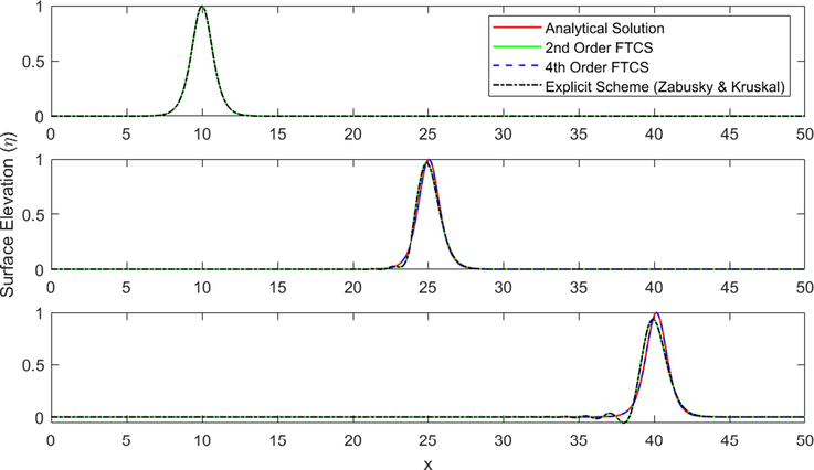

Close

Fig. 2

Comparisons between analytical solutions, 2nd-Order and 4th-Order Finite Difference (FTCS) Scheme, as well as modified Explicit Scheme from Zabusky and Kruskal (1965) in simulating wave propagation over a flat bottom with $\alpha =0.01,\beta =0.00625,\delta =0\text{.}$ , and $A=1$ .

Export to PPT

Fig. 2 shows an extremely good agreement between the numerical result and analytical solution of solitary wave propagation over a flat bottom. Our computational scheme has approximated the solitary wave amplitude and speed accurately, without any sign of dissipation, while still managed to keep the wave shape during the observation. On the contrary, notice that the numerical results obtained using a modified scheme from Zabusky and Kruskal (1965) display an amplitude dissipation throughout the observation. Even though the speed is simulated nicely, the scheme could not maintain the wave shape, and instead, caused a distortion to be displayed in the simulation. Similar results obtained using a 2nd-Order FTCS scheme, indicating that the 4th-Order FTCS is significantly more accurate than the 2nd-Order scheme. Even though, 2nd-Order scheme would be slightly faster in simulating KdV equation, but the accuracy is much more important in this case, since it affects the wave shape and amplitude. Therefore, in this case, we can say that our 4th-Order FTCS scheme works better than the 2nd-Order FTCS scheme and the modified explicit scheme from Zabusky and Kruskal (1965). And since our numerical scheme has also been validated by the analytical solutions, we can use our numerical scheme to investigate further cases, the first one being wave shoaling scenario.

To model a shoaling occurrence, we need to define an uneven bottom height $h(x)$ that goes from deeper to shallower depth along the spatial axis. In this case, since our model is only applicable for $h(x)=\mathit{kx}$ , we define the water depth as three sub-domains. The first sub-domain, being the deepest domain is a flat bottom, thus, the slope is $k_1=0$ . The second sub-domain is the transition domain with a slope of $k_2\ne 0$ . The shallower sub-domain, which is the third one, is also a flat bottom with different value of depth. Mathematically, this domain can be written as

For this simulation, we set a different observation domain, which is $x\in [0,100]$ , with partition length of $\mathrm{\Delta }x=0.1$ and time step of $\mathrm{\Delta }t=0.001$ . Thus, the number of the partitions is 1000. For the characteristics of the initial solitary wave, we use the same initial condition which is $\eta (x,t)=A{\mathrm{sech}}^2\left(\sqrt{\frac{3}{4}\frac{\alpha }{\beta }A}\left(x-10\right)\right)$ with $A=1$ . The other parameters are set to be $\alpha =0.01$ and $\beta =0.01$ . Since now we are studying the case where the bottom topography is uneven, the value of small parameter $\delta$ is not zero, or in this case, we fix $\delta =0.7$ . Further, in this specific case, we choose the depth to be $h_0=-2$ and $h_1=-1.5$ , whereas the starting and ending point of the slope is $x_0=20$ and $x_1=70$ , respectively. It means, the width of the slope is 50. This set-up implies that the slope is fixed with the value of $k_2=0.01$ . Using the computational scheme as in Eq. (12), we simulate wave propagation over the topography $h(x)$ in which result can be seen in Fig. 3.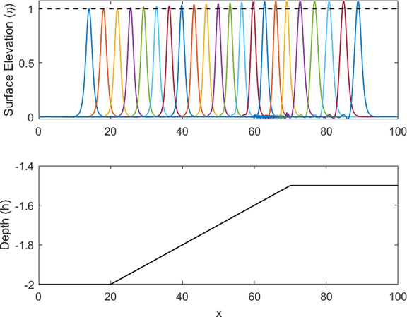

Close

Fig. 3

Wave shoaling simulation for soliton with $\alpha =0.01,\beta =0.01,\delta =0.7,A=1$ , and $k_2=0.01$ .

Export to PPT

From Fig. 3, it can be clearly seen that the solitary wave undergoes a shoaling phenomenon right when it enters the sloping domain. It is indicated by the rise in its amplitude, and, even though it is not visible in the figure, the decrease of its wavelength. Right after the wave passes over the slope and starts to enter the flat bottom domain again, it is noticeable that the amplitude is back to being constant. A slight distortion shown in the figure when the wave starting to enter the shallower domain is might be appeared due to the supposedly reflected part of the wave. When a wave enters a shallower domain with a sudden depth change in the domain, it is natural that the wave will be divided into two separate parts, the one transmitted onward to the coast and the one reflected bach to the open ocean. However, in KdV-type equation, we can only explain a wave moving to only one direction, meaning that the equation cannot capture both transmitted and reflected wave accurately. Thus, in this case, the reflected wave is captured as a distortion of the main wave, which is the transmitted wave.

However, in this specific scenario, this does not matter at all, since we can still estimate the wave amplitude correctly. It is proven by comparing the numerical shoaling coefficient to its analytical counterpart. The analytical wave shoaling coefficient is defined as $K_s={\left(\frac{h_0}{h_1}\right)}^{1/4}$ (Kajiura, 1961). The numerical wave shoaling coefficient is calculated using $K_s^{\mathit{num}}=\frac{\mathit{max}\left(\eta \right)}{A}$ . The value of $\mathit{max}(\eta )$ is calculated on the last domain only, which the shallower flat domain, after the wave passes the slope. Using these formulations, it is found from the first simulation that the relative error between analytical and numerical wave shoaling coefficient is $\mathit{error}=\left|(\frac{K_s-K_s^{\mathit{num}}}{K_s})\right|=0.16\%$ . This error in an extremely small value of error, which implies that our numerical scheme has successfully estimated the analytical wave shoaling coefficient, and therefore, accurately simulated the wave shoaling phenomenon.

Next, we move on to the further investigation of the model. This time, we will perform several simulations to investigate the effect of slope height and width on the wave shoaling coefficient which results will be compared to the analytical coefficient. First, we start with the observation of how changing the slope height affects the wave shoaling coefficient. We use the same spatial domain, which is $x\in [0,100]$ , with also the same partition length and time step, which are $\mathrm{\Delta }x=0.1$ and $\mathrm{\Delta }t=0.0001$ , respectively. The initial condition and small parameters are still the same. However, in this case, we fix the deeper water depth to be $h_0=-2$ , while the shallower one is varied within the range of $h_1\in [-2,-1.4]$ . The slope width is also fixed at 50. The comparison of the numerical and analytical wave shoaling coefficient for different slope height is presented in Fig. 4.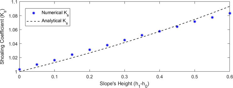

Close

Fig. 4

Comparison between the numerical and analytical wave shoaling coefficient for different slope height with $\alpha =0.01,\beta =0.01$ , and $\delta =0.7$ .

Export to PPT

In Fig. 4, it can be seen that the wave shoaling coefficient $(K_s)$ increases as the slope height rises. In other words, the shallower the domain behind the slope, the bigger the value of wave shoaling phenomenon. This confirms the actual characteristic of wave shoaling, which has also been confirmed by previous researches using different models or methods (Magdalena and Iryanto, 2018). From these simulations, we can also calculate the average relative error between the numerical and analytical $k_s$ , which is $\mathit{average}\mathit{error}=0.38\%$ , which is a quite small error for shallow water simulations.

Following the investigation regarding slope height effect on wave shoaling, we will also study how slope width affects the wave shoaling coefficient $(K_s)$ . We use the exactly same spatial domain, partition length, and time step as the previous simulations. We will also use the same initial condition and initial amplitude. The difference here is that we fix the water depth at the value of $h_0=-2$ for the deeper area and $h_1=-1.8$ for the shallower region. The starting point of the slope is set to be $x_0=30$ , with slope width varies within the range of $\mathit{width}\in [20,40]$ . We will perform simulations on this configuration using our computational model and compare the results to the analytical wave shoaling coefficient. The comparison is shown in Fig. 5.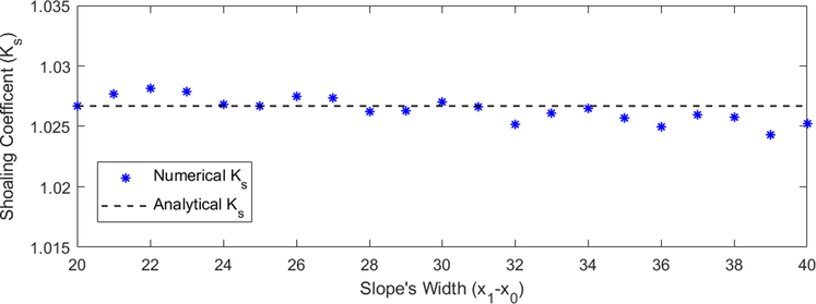

Close

Fig. 5

Comparison between the numerical and analytical wave shoaling coefficient for different slope width with $\alpha =0.01,\beta =0.01$ , and $\delta =0.6$ .

Export to PPT

In Fig. 5, it is shown that the wave shoaling coefficient is not significantly affected by the changes in slope width. This confirms the analytical formula for wave shoaling coefficient, which is $K_s={\left(\frac{h_0}{h_1}\right)}^{1/4}$ . It is clear in the formula that only the water depths affect the shoaling coefficient, while the slope width, or can also be interpreted as the slope $k_2$ , does not have any effect on the coefficient. This is why, in the numerical simulations, even though the values of $K_s$ are fluctuate as the slope width changes, but they are still in the close proximity with each other, meaning that in general, we can say that the values of $K_s$ are relatively constant. This statement is proved by the average relative error between the numerical and analytical $K_s$ , which is around $0.079\%$ .

The next issue to be addressed is the distortion that was mentioned previously. As explained before, the distortion appeared in the simulations are most likely due to the reflected wave that cannot be captured correctly. This distortion is even more visible as the domain after the slope becomes shallower. This is because the shallower the domain behind the slope, the more significant it affects the wave, therefore, the distortion might become more visible. This also can be happened when the slope is steep enough to significantly affect the wave. To illustrate this explanation, we perform and compare two simulations results, one of which is for smaller slope (deeper $h_1$ ) and another one is for steeper slope (shallower $h_1$ ). The results are presented in Figs. 6 and 7.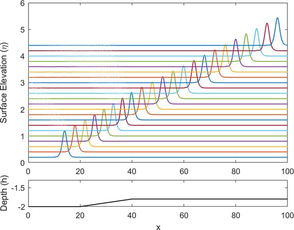

Close

Fig. 6

Wave shoaling simulation over a smaller slope where there is no distortion produced ( $\alpha =0.01,\beta =0.01,\delta =0.7,A=1,\mathit{slope}\mathit{width}=20,h_0=-2$ , and $h_1=-1.8$ ).

Export to PPT

Close

Fig. 7

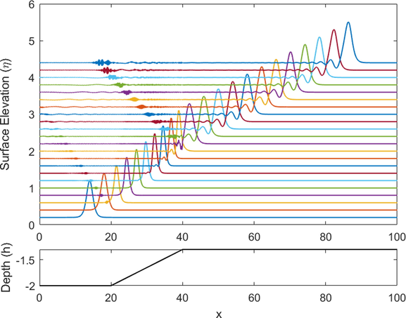
Wave shoaling simulation over a steeper slope where distortion is clearly visible ( $\alpha =0.01,\beta =0.01,\delta =0.7,A=1,\mathit{slope}\mathit{width}=20,h_0=-2$ , and $h_1=-1.3$ ).

Export to PPT

Fig. 6 shows wave shoaling phenomenon over a slope when the depth of the area after the slope is not too deep, thus, the slope is also not too steep. Meanwhile, Fig. 7 illustrates the same simulation when the region after the slope is shallower, indicates that the slope is steeper. Now, notice how different the model capture both simulations. In Fig. 6, it can be seen that there is no distortion generated. This is because the change in the topography is extremely small that it will not affect the wave significantly, hence, the wave amplitude is also not affected much. It means that the reflected wave is actually still there but it is hardly possible to be noticed visually. On the other hand, we can clearly see the distortion in Fig. 7 which slope is much steeper than in Fig. 6. The distortion is generated at two different positions, which are at the start and the end of the slope. However, at the start of the slope, the distortion is much smaller than the one at the end of the slope. This is due to the difference in water depths. At the starting point, the depth is still deep enough, while at the ending point, the water depth is much shallower. As mentioned before, the shallower the depth, the more it affect the wave amplitude, which also will generate more reflected wave, which is then captured as distortion. Moreover, both distortions travel to the opposite direction of the actual wave, since it is actually reflected by the slope. However, the distortion speed might not be the same as the wave speed.

Apart from the distortion, we also notice how the wave starts to reduce its length when it enters the slope. The wavelength becomes smaller as the wave propagates over the slope, hence, the amplitude becomes higher. At the same time, the wave speed becomes slower when the wave enters the slope, indicated by a small deflection in the wave movement. This speed is then brought back to a faster one after it passes over the slope, indicated by the positive deflection in the movement. It confirms one of the characteristics of wave shoaling, which is the wave becomes slower as it travels over a slope and becomes faster as it escapes the slope. In addition, we can see that there is a change in the shape of the wave. The wave, which once has a smooth solitary wave form, changes to a more complex wave consists of more than one wave. This might be happened due to the distortion that occurred previously.

6 Conclusion

Shoaling wave propagation over a sloping topography has been modeled using the KdV-type equation that was previously developed. An analytical solution to the equation was derived for the flat bottom case. Meanwhile, in the case of uneven bottom topography, a numerical scheme is used to simulate the equation. The numerical scheme was developed using the 4th-Order Finite Difference method, particularly by applying the Forward Time and Centered Space approach. To validate the scheme, the simulation results are compared to the analytical solutions, results of the 2nd-Order Finite Difference method, as well as the Explicit Method that was established prior to this research. The comparisons are performed for solitary wave propagation over a flat bottom. It is shown that the 4th-Order Finite Difference scheme approximates the analytical solution better than the other two methods. Furthermore, shoaling wave propagation is simulated, where the numerical shoaling coefficient is found to be in agreement with the analytical shoaling coefficient with an error of $0.16\%$ . The effects of the height and width of the sloping bottom on the shoaling coefficient are then explored and compared to their analytical counterparts. The results show that the change in the slope’s height is directly proportional to the shoaling coefficient, while the slope’s width has no significant effect on the coefficient. In both cases, the comparisons between analytical and numerical approaches give less than $0.4\%$ error. Apart from the shoaling coefficients, the change in slope’s height can also affect the shape of the solitary wave. As the slope becomes higher (the slope becomes steeper), the wave starts to show a distortion in its shape which will travel in the opposite direction as the wave.

References

- A formal derivation and numerical modelling of the improved boussinesq equations for varying depth. Ocean Eng.. 1996;23:691-704.
- [Google Scholar]
- Surface waves propagation in shallow water: A finite element model. Int. J. Numer. Meth. Fluids. 1993;16:447-459.
- Numerical study on regular wave shoaling, de-shoaling and decomposition of free/bound waves on gentle and steep foreshores. J. Marine Sci. Eng.. 2020;8
- One- and two-soliton solutions to a new kdv evolution equation with nonlinear and nonlocal terms for the water wave problem. Nonlinear Dyn.. 2016;83:2461-2473.
- Fully nonlinear model for water wave propagation from deep to shallow waters. J. Waterway Port Coastal Ocean Eng.. 2012;138:362-371.
- Calculation of solitary wave shoaling on plane beaches by extended boussinesq equations. Eng. Appl. Comput. Fluid Mech.. 2012;6:25-38.
- Shoaling of solitary waves on plane beaches. J. Waterway Port Coastal Ocean Eng.. 1994;120:609-628.
- Kajiura, K., 1961. On the partial reflection of water waves passing over a bottom of variable depth. In: Proceedings of the Tsunami Meetings 10th Pacific Science Congress, IUGG, pp. 206–234.
- Can simple kdv-type equations be derived for shallow water problem with bottom bathymetry? Commun. Nonlinear Sci. Numer. Simul.. 2020;82:105073.
- A new form of the boussinesq equations with improved linear dispersion characteristics. Part 2. a slowly-varying bathymetry. Coast. Eng.. 1992;18:183-204.
- A new boussinesq method for fully nonlinear waves from shallow to deep water. J. Fluid Mech.. 2002;462:1-30.
- Reeve, Free-surface long wave propagation over linear and parabolic transition shelves. Water Sci. Eng.. 2018;11:318-327.
- Effects of viscosity and surface tension on soliton dynamics in the generalized kdv equation for shallow water waves. Commun. Nonlinear Sci. Numer. Simul.. 2021;102:105942.
- Alternative form of boussinesq equations for nearshore wave propagation. J. Waterway Port Coastal Ocean Eng.. 1993;119:618-638.
- Velocity predictions for shoaling and breaking waves with a boussinesq-type model. Coast. Eng.. 2000;41:361-397.
- Linear shoaling in boussinesq-type wave propagation models. Coast. Eng.. 2013;80:100-106.
- Wave shoaling over a submerged ramp: An experimental and numerical study. J. Waterway Port Coastal Ocean Eng.. 2018;144
- Tsunamis, 2021. URL: https://www.who.int/health-topics/tsunamis.
- Tsunami shoaling, 2011. URL: https://www.sciencelearn.org.nz/resources/596-tsunami-shoaling.
- UNDRR, Tsunamis account for $280 billion in economic losses over last twenty years - world, 2018. URL: https://reliefweb.int/report/world/tsunamis-account-280-billion-economic-losses-over-last-twenty-years.
- A conservative fourth-order stable finite difference scheme for the generalized rosenau–kdv equation in both 1d and 2d. J. Comput. Appl. Math.. 2019;355:310-331.
- Interaction of solitons in a collisionless plasma and the recurrence of initial states. Phys. Rev. Lett.. 1965;15:240-243.
- A new form of generalized boussinesq equations for varying water depth. Ocean Eng.. 2004;31:2047-2072.