Numerical solution of singular boundary value problems using Green’s function and Sinc-Collocation method

1 Introduction

We consider a class of nonhomogeneous SBVPs:

If $P\left(x\right)$ has singularity at $x=0$ such as $P\left(x\right)=\frac{\beta }{x}$ with $\beta >0$, then the problems (1)–(2) is called Lane-Emden type equations. We assume that constants $a_0$ and $a_1$, and likewise $b_0$ and $b_1$, both are not zero. The unique solution of problems (1) subjected to the boundary conditions (2) is depend on the following conditions on $P\left(x\right),Q\left(x\right)$, and $R\left(x\right)$:

• E1. Let $P\left(x\right)$ is measurable on $[0,1]$ and continuous on $(0,1]$;

• E2. $P\left(x\right)>0$ on $(0,1]$;

• E3. ${\int }_0^1\mathit{xP}\left(x\right)<\infty$;

• E4. Let $Q\left(x\right)$ is continuous on $[0,1]$.

The Lane-Emden equations is the model for several phenomena in physics and astrophysics Parand and Pirkhedri, 2010; Wazwaz, 2011; Yuzbası and Sezer, 2013.

Many researchers have tried to solve problems (1)–(2) numerically. Mohanty et al. Mohanty et al., 2004 using cubic spline method for solving SBVPs. Variational iteration scheme by Wazwaz Wazwaz, 2011. Pirabaharan et al. Pirabaharan and Chandrakumar, 2016 discussed a new Bernstein polynomials method. The modified Bessel Collocation by Suayip Yuzbası, et al. Yuzbası and Sezer, 2013.

The Sinc function is widely used in various numerical methods which introduced by F. Stenger Stenger, 1993; Stenger, 2011. Rashidinia Rashidinia and Nabati, 2013; Rashidinia and Taheri, 2015 used Sinc methods based on Sinc function for SBVPs.

The Green’ function is used for solving BVPs in one, two, and three dimensionalRahman, 2007. Z. Cen Cen, 2006 used Green’s function to developed equivalent integral equation for SBVPs. Singh et al. Singh et al., 2013 using Adomian decomposition and Green’s function.

In this paper, we apply a new direction for approximating the nonhomogeneous SBVPs (1)–(2) which can be reduced to a Volterra-Fredholm integral equation with the help of Green’s function. In our approach, the convergence accuracy of the solution is $O\left(e^{(-\vartheta \sqrt{N})}\right)$, where $\vartheta >0$, and also converges at an optimal rate, because the singularity on the boundary of approximation is ignoredRashidinia and Zarebnia, 2007; Rashidinia and Zarebnia, 2007.

Section 2 deals with representation of the solution of the SBVPs (1)–(2) by Green’s function. In Section 3, after some preliminary definitions and theorems of Sinc function, the Sinc-Collocation method has been used to replace Volterra-Fredholm integral equation corresponding to problems (1)–(2). The converges of the methods are considered in Section 4. Finally, three test examples are presented in Section 5 and the conclusion is considered in the rest of the section.

2 Representation of the Green’s function

The method of variation of parameter is used to construct Green’s function for an integral representation of nonhomogeneous SBVPs (1)–(2). First of all, we convert the nonhomogeneous boundary conditions (2) to homogeneous Stenger, 1993, then we define an interpolating boundary function

Consequently, the problems (1)–(2) reduce to the following problem:

The homogeneous part of Eqs. (5) is:

Let $u_1\left(x\right)$ and $u_2\left(x\right)$ be two solutions of problem (7) which are linearly independent. By using variation of parameters (see Rahman, 2007), the Green’s function of (5) and (6) can easily be constructed as:

It is obvious that $G(x,t)$ is matched with boundary conditions (6). The properties of the $G(x,t)$ are summarised in appendix A.

Now, by using (8), a particular solution of Eqs. 5,6 in integral form can be obtained as:

The proof of Eq. (10) is in the appendix B.

3 Sinc function preliminaries and the Sinc-Collocation method

We first introduce some preliminaries of Sinc function, Sinc interpolation Stenger, 1993; Stenger, 2011 that are important here, and then we discussed the Sinc-Collocation method.

4 Convergence analysis

By the following theorem, we proof that the Volterra-Fredholm Eq. (9) has the unique solution.

Theorem 4. We consider the assumptions (E1)-(E4), and Green’s function 8, so we have.

• I.$m_1≔{\max }_{0⩽x⩽1}\left|{\int }_0^{1}G\right(x,t\left)\mathit{dt}\right|<\infty$,

• II. $m_2≔{\max }_{0⩽x⩽1}\left|{\int }_0^{1}P\right(x\left)G_x\right(x,t\left)\mathit{dt}\right|<\infty$.

Proof. (i) The proof is clear. It follows from the Green’s function (8) and the assumptions (E1)-(E4).(ii) For $G_x(x,t)=\frac{\partial G(x,t)}{\partial x}$, we have$$G_x(x,t)=\left\{\begin{array}{c}\frac{u_1^{\prime }\left(x\right)u_2\left(t\right)}{W\left(t\right)},t⩽x⩽1,\hfill \\ \frac{u_2^{\prime }\left(x\right)u_1\left(t\right)}{W\left(t\right)},0⩽x⩽t\text{.}\hfill \end{array}\right.$$

Hence,

Because, $G(x,t)$ satisfies the differential Eq. (5) as follows:

Hence, from (23) we have$$P\left(x\right)G_x(x,t)=\left\{\begin{array}{c}0,0⩽x⩽t⩽1,\hfill \\ -1,0⩽t⩽x⩽1\text{.}\hfill \end{array}\right.$$

Hence, we obtain $c={\max }_{0⩽x,t⩽1}\left|P\right(x\left)G_x\right(x,t\left)\mathit{dt}\right|<\infty$, and then.

$m_2={\max }_{0⩽x,t⩽1}\left|{\int }_{t^{-0}}^{t^{+0}}P\right(x\left)G_x\right(x,t\left)\right|⩽c<\infty$.

Theorem 5. We assume that $u_m\left(x\right)$ and $u\left(x\right)\in L_{\alpha }\left(\mathcal{D}\right)$ are the approximate and exact solutions of integral Eq. (10) respectively. Suppose that all conditions of Theorems 1, 2, and 3 are fulfilled. By considering $h={(\pi d/(\alpha N\left)\right)}^{1/2}$ and $\frac{u}{{\phi }^{\prime }}\in L_{\alpha }\left(\mathcal{D}\right),(\alpha >0)$, there exist a constant $\zeta >0$ , so$${\displaystyle \underset{0⩽x⩽1}{\max }}\left|u\right(x)-u_m(x\left)\right|<\zeta e^{{(\pi d/(\alpha N\left)\right)}^{1/2}}\text{.}$$

Proof. Using the relations (11), (15), and (17), we have$$\begin{array}{cc}\left|e_m\right(x\left)\right|\hfill & ={\displaystyle \underset{0⩽x⩽1}{\max }}\left|u\right(x)-u_m(x\left)\right|\hfill \\ \hfill & ⩽{\displaystyle \underset{0⩽x⩽1}{\max }}\left|u\right(x)-\left(c_{-N-1}{\varpi }_0\left(x\right)+{\displaystyle \sum _{j=-N}^{}}{\mathit{Nc}}_j{\mathrm{\Theta }}_j\left(\phi \right(x\left)\right)+c_{N+1}{\varpi }_1\left(x\right)\right)|\hfill \\ \hfill & +|-u_1(x){\int }_0^x\frac{u_2\left(t\right)f\left(t\right)}{W\left(t\right)}\mathit{dt}+h{\displaystyle \sum _{j=-N}^N}\frac{{\delta }_{\mathit{kj}}^{(-1)}}{{\phi }^{\prime }\left(t_j\right)}\frac{u_1\left(x_k\right)u_2\left(t_j\right)f\left(t_j\right)}{W\left(t_j\right)}|\hfill \\ \hfill & +\left|u_2\right(x){\int }_0^x\frac{u_1(t+1)f(t+1)}{W(t+1)}\mathit{dt}-h{\displaystyle \sum _{j=-N}^N}\frac{{\delta }_{\mathit{kj}}^{(-1)}}{{\phi }^{\prime }\left(t_j\right)}\frac{u_2\left(x_k\right)u_1(t_j+1)f(t_j+1)}{W(t_j+1)}|\hfill \\ \hfill & +|-u_2(x){\int }_0^1\frac{u_1(t+x)f(t+x)}{W(t+x)}\mathit{dt}+h{\displaystyle \sum _{j=-N}^N}\frac{u_2\left(x_k\right)u_1(t_j+x_k)f(t_j+x_k)}{{\phi }^{\prime }\left(t_j\right)W(t_j+x_k)}|\hfill \\ \hfill & ⩽k_1{e}^{{(\pi d/(\alpha N\left)\right)}^{1/2}}+k_2{e}^{{(\pi d/(\alpha N\left)\right)}^{1/2}}+k_3{e}^{{(\pi d/(\alpha N\left)\right)}^{1/2}}\hfill \end{array}$$

By considering $\zeta =\max \{k_1,k_2,k_3\}$, we have$$\left|e_m\right(x\left)\right|⩽\zeta e^{{(\pi d/(\alpha N\left)\right)}^{1/2}}$$then the proof is completed.

Theorem 5 demonstrates that the mentioned method converges at the rate of $O\left(e^{-\vartheta \sqrt{N}}\right)$, where $\vartheta >0$.

5 Numerical results

In this section, three examples are presented based on the Green’s function and the Sinc-Collocation method Parand and Pirkhedri, 2010; Yuzbası and Sezer, 2013 for illustrating the effectiveness and importance of the proposed method. All experiments were performed in Mathematica 11.0. Also, in order to show the errors and the accuracy of the approximation, on the set of sinc grid points$$S=\{x_{-N-1},x_{-N},\dots ,x_N,x_{N+1}\},$$$$x_k=\frac{e^{\mathit{kh}}}{1+e^{\mathit{kh}}},k=-N-1,-N,\dots ,N,N+1,$$we apply the following criteria:

• 1. The relative error is defined by

  (25)

  $$E_{\mathit{rel}}=\left|\frac{u_m\left(x_k\right)-u\left(x_k\right)}{u\left(x_k\right)}\right|\text{.}$$

• 2. The maximum absolute error is defined by

  (26)

  $$E_{\mathit{abs}}={\displaystyle \underset{-N-1⩽k⩽N+1}{\max }}\left|u\right(x_k)-u_m(x_k\left)\right|\text{.}$$

• 3. The root mean square (RMS) error is defined for $M=2N+3$ by

  (27)

  $$\mathit{RMS}=\sqrt{\frac{1}{M}{\displaystyle \sum _{k=-N-1}^{N+1}}{\left(u\left(x_k\right)-u_m\left(x_k\right)\right)}^2}\text{.}$$

• 4. The $L_2$ error norm is defined by

  (28)

  $$\left|\right|.|{|}_2=\sqrt{{\displaystyle \sum _{k=-N-1}^{N+1}}{\left(u\right(x_k)-u_m(x_k\left)\right)}^2}\text{.}$$

In our presented method, we take $d=\frac{\pi }{2},\alpha =1$ and we applied our procedure for $N=10,20,30,40$, and 50 and by using $h={(\pi d/(\alpha N\left)\right)}^{1/2}$ we can achieve h. The consistency of approximate and exact solution is shown in the Figures. By increasing N, the errors have been decreased in the Tables.

Example 1. We consider the following SBVP:$$\left\{\begin{array}{c}{y}^{″}\left(x\right)-\frac{3}{x}{y}^{\prime }\left(x\right)=3x,x\in [0,1]\hfill \\ y\left(0\right)=y\left(1\right)=0\text{.}\hfill \end{array}\right.$$

This problem has the exact solution $y\left(x\right)=x^4-x^3$, and by using (8) the Green’s function is:$$G(x,t)=\left\{\begin{array}{c}\frac{t^4(1-x^4)}{4t^3},0⩽t⩽x\text{;}\hfill \\ \frac{x^4(1-t^4)}{4t^3},x⩽t⩽1\text{.}\hfill \end{array}\right.$$

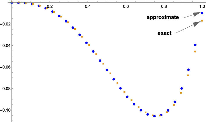
By increasing N, we tabulated the relative errors (25) in Table 1. Table 2 lists the errors (26)–(28). The graph of the approximate and exact solutions is in Fig. 1 which are coincide together. Fig. 2, illustrates LogPlot of the relative errors. In this example, we have $\mathit{Cond}\left(A\right)=\Vert A\Vert \Vert A^{-1}\Vert =1$ in the system (22) for a list of N.

Close

Fig. 1

Comparison between the exact and approximate solutions of Example 1 with $N=10$.

Export to PPT

Close

Fig. 2

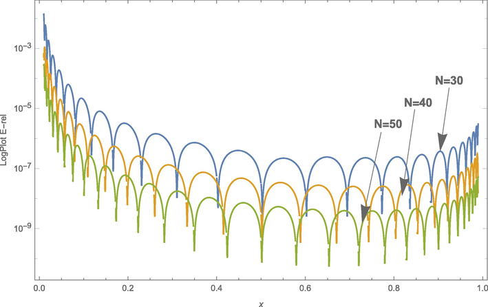
LogPlot of the relative errors of Example 1 with different values of N.

Export to PPT

Example 2. We consider the following SBVP:$$\left\{\begin{array}{c}{y}^{″}\left(x\right)+\frac{2}{x}{y}^{\prime }\left(x\right)+1=0,x\in [0,1]\hfill \\ 6y\left(1\right)+3y^{\prime }\left(1\right)=4,y\left(0\right)=1\text{.}\hfill \end{array}\right.$$

The exact solution is: $y\left(x\right)=1-\frac{x^2}{6}$. This may be transformed into the following form with homogeneous boundary conditions. If we use the relations (3) and (4), then we have:$$\left\{\begin{array}{c}{u}^{″}\left(x\right)+\frac{2}{x}{u}^{\prime }\left(x\right)=\frac{4}{9x}-1,x\in [0,1]\hfill \\ u\left(0\right)=0,6u\left(1\right)+3u^{\prime }\left(1\right)=0\text{.}\hfill \end{array}\right.$$

By using (8), the Green’s function is$$G(x,t)=\left\{\begin{array}{c}(\frac{-1}{2}+\frac{1}{x})(-t^2),0⩽t⩽x\text{;}\hfill \\ (\frac{-1}{2}+\frac{1}{t})(-t^2),x⩽t⩽1\text{.}\hfill \end{array}\right.$$

By increasing N, we tabulated the relative errors (25) in Table 3. Table 4 is consist of list of the errors (26)–(28), and Cond$\left(A\right)$. The log–log plot of the approximate and exact solutions is in the Fig. 3.

Close

Fig. 3

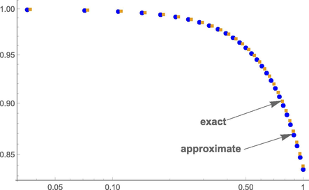
Log–LogPlot of the exact and approximate solutions of Example 2 with $N=10$.

Export to PPT

Example 3. We consider the following SBVP:$$\left\{\begin{array}{c}{y}^{″}\left(x\right)+\frac{2}{x}{y}^{\prime }\left(x\right)-4y=-2,x\in [0,1]\hfill \\ y^{\prime }\left(0\right)=1,y\left(1\right)=5.5,\hfill \end{array}\right.$$

The exact solution is: $y\left(x\right)=0.5+\frac{5\sinh \left(2x\right)}{x\sinh \left(2\right)}$. By using (8), the Green’s function is$$G(x,t)=\left\{\begin{array}{c}\frac{5e^4}{1-e^4}(-\frac{e^{2x}{e}^{-4}}{x}+\frac{e^{-2x}}{x})(\frac{e^{2t}}{t}-\frac{e^{-2t}}{t})t^2,0⩽t⩽x\text{;}\hfill \\ \frac{5e^4}{1-e^4}(\frac{e^{2x}}{x}-\frac{e^{-2x}}{x})(-\frac{e^{2t}{e}^{-4}}{t}+\frac{e^{-2t}}{t})t^2,x⩽t⩽1\text{.}\hfill \end{array}\right.$$

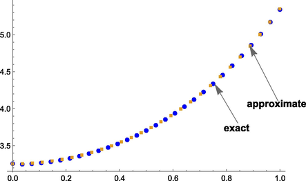
By increasing N, we tabulated the relative errors (25) in Table 5 and Table 6 is consist of list of the errors (26)–(28), and Cond$\left(A\right)$. Fig. 4 shows the graph of the approximate and exact solutions which are coincide together.

References

- Numerical study for a class of SBVPs using Green’s functions. Appl. Math. Comput.. 2006;183:10-16.
- [Google Scholar]
- An accurate cubic spline TAGE method for nonlinear SBVPs. Appl. Math. Comput.. 2004;158:853-868.
- A computational method for solving a class of SBVPs arising in science and engineering. Egypt. J. Basic Appl.. 2016;sciences,3:383-391.
- Sinc-Collocation method for solving astrophysics equations. J. New Astron.. 2010;15:533-537.
- Integral Equations and their Applications. Canada: Dalhousie University; 2007.
- Sinc-Galerkin and Sinc-Collocation methods in the solution of nonlinear two-point BVPs. Comp. Appl. Math.. 2013;32:315-330.
- Convergence of approximate solution of system of Fredholm integral equations. J. Math. Anal.. 2007;333:1216-1227.
- Solution of a Voltera integral equation by the sinc-Collocation method. J. Comput. Appl. Math.. 2007;206:801-813.
- Sinc methods involving exponential transformations to solve Lane-Emden type equations. J. Afr. Mat.. 2015;27:541-554.
- Numerical solution of SBVPs using Green’s function and improved decomposition method. J. Appl. Math. Comput.. 2013;43:409-425.
- Numerical Method Based on Sinc and Analytic Functions. New York Inc: Springer-Verlag; 1993.
- Handbook of Sinc Numerical Methods. Boca Raton: CRC Press; 2011.
- The variational iteration method for solving nonlinear SBVPs arising in various physical models. Commun. Nonlin. Sci. Num. Simult.. 2011;16:3881-3886.
- An improved Bessel collocation method with a residual error function to solve a class of Lane-Emden differential equations. J. Math. Comput. Modell.. 2013;57 1298–131
Appendix A
The properties of the are summarised as follows: I. Boundary conditions: II. The condition of Continuity: III. Jump discontinuity of the gradient:
Then a solution of the given BVPs (5)–(6) can be obtained as: