Numerical solution for the Kawahara equation using local RBF-FD meshless method

1 Introduction

Nonlinear evolution equations play an essential role in engineering and mathematical physics such as solid state physics, fluid mechanics, chemical physics, plasma physics, geochemistry and chemical kinematics fields (Ablowitz et al., 1991; Jeffrey and Xu, 1989; Raslan and EL-Danaf, 2010; Mohanty and Gopal, 2011; Sharifi and Rashidinia, 2019; Mohanty and Khurana, 2019; Nikan et al., 2019). One of the well-known nonlinear evolution equations is the fifth order Kawahara equation which is appeared in the theories of shallow water waves having surface tension, magneto-acoustic waves in a plasma and capillary-gravity waves (Korkmaz and Dağ, 2009; Sirendaoreji, 2004). In this study, we consider the Kawahara equation (Ceballos et al., 2007) in the following form

Where $V=V(x,t)$; and $g,h_a,h_b$ are known functions and $\mu$ and $\rho$ are known coefficients.

In special forms of the Kawahara equation, the analytical solution in the case of solitary waves is studied by some researchers (Sirendaoreji, 2004; Yamamoto and Takizawa, 1981; Yusufoğlu et al., 2008). Generally, obtaining the analytic solution for the nonlinear differential equations is not possible, so the numerical approximations are necessary for solving such models (Bashan et al., 2017; Başhan, 2019; Başhan, 2019). The numerical solution of the Kawahara equation has been investigated by many researchers (Korkmaz and Dağ, 2009; Djidjeli et al., 1995; Ceballos et al., 2007; Haq and Uddin, 2011; Abazari and Soltanalizadeh, 2012; Gong et al., 2014; Karakoc et al., 2014; Başhan, 2019). Also, some other methods based on homotopy analysis are proposed for the approximate solution of the Kawahara equation (Abbasbandy, 2010; Wang, 2011; Kashkari, 2014).

In recent years, RBFs meshfree collocation techniques have been extensively used for obtaining the numerical solutions of PDEs (Sarra, 2005; Meshfree, 2007; Hussain and Haq, 2020; Dereli et al., 2009; Bibi et al., 2011; Safdari-Vaighani and Mahzarnia, 2015). Some of the major advantages of RBFs approaches are spectral convergence rates, computing derivatives, geometrical flexibility and the ease of applying in high dimensions. Although RBFs methods have a spectral accuracy, they often have a large linear system with full and ill-conditioned matrices. To overcome such difficulties, the local RBF-FD method was investigated by some authors (Wright and Fornberg, 2006; Bayona et al., 2010; Martin and Fornberg, 2017; Dehghan and Mohammadi, 2017; Dehghan and Abbaszadeh, 2017; Nikan et al., 2019; Rashidinia and Rasoulizadeh, 2019). This method has a sparse and well-conditioned system.

The main purpose of this manuscript is to develop the local RBF-FD method to solve the Kawahara equation as a time-dependent PDEs. In addition, a comparison between proposed method and the methods MQ and $r^7$ RBFs (Haq and Uddin, 2011), CDQ and PDQ (Korkmaz and Dağ, 2009), and MCBC-DQM (Başhan, 2019) is given.

The rest of the present study is as follows; In Section 2, the RBFs and RBF-FD collocation methods will be reviewed briefly. In Section 3, a description of the meshless RBF-FD method to compute the numerical solution of the Kawahara equation is given. In Section 4, the stability analysis of the proposed method is proved. In Section 5, the numerical experiments is reported.

2 Collocation methods

Let $X=\{{\underline{x}}_1,{\underline{x}}_2,\cdots ,{\underline{x}}_N\}\subseteq {\mathbb{R}}^d$, be a set of N separate points with known scalar values $f_i$ for $i=1,2,\dots ,N$.

3 Description of the method

The implementation details of the RBF-FD method for the Kawahara equation are described in this section.

First, $m+1$ distinct points $t_k=k\tau ,k=0,1,\cdots ,m$, on interval $[0,T]$ with time step size $\tau$ are chosen. Then, the finite difference (FD) and $\theta$-weighted $(0⩽\theta ⩽1)$ methods are applied over two consecutive time steps $t_k$ and $t_{k+1}$ on Eq. (1) as

The nonlinear term ${(V\frac{\partial V}{\partial x})}^{k+1}$ can be approximated by linear term (Rashidinia and Rasoulizadeh, 2019) as

After substituting Eq. (9) into Eq. (8), it can be written as

Now, N distinct collocation nodes $X=\left\{x_1,x_2,\cdots ,x_N\right\}$ are chosen in the interval $[a,b]$ in which $x_i,i=2,\cdots ,N-1$ are the $N-2$ interior nodes and $x_i,i=1,N$ are the 2 boundary nodes.

For each point $x_i$, stencil $I_i=\left\{x_j\in X:\mid x_j-x_i\mid ⩽R\right\}=\left\{x_{i_1},x_{i_2},\cdots ,x_{i_{n_i}}\right\}$ in its support radius R is chosen. Without loss of generality, let us assume $x_i=x_{i_1}(i=i_1)$. For each node $x_i$ and its stencil $I_i$, the weights ${\underline{w}}_{\mathit{sx},i}={[w_{\mathit{sx},i1},\cdots ,w_{\mathit{sx},{\mathit{in}}_i}]}^T$ corresponding to $\frac{{\partial }^s}{\partial x^s}$ for $s=1,3$, and 5 will be determined by using RBF-FD method Eq. (6). Thus we obtain

Eq. (12) along with the boundary conditions Eq. (1c), lead to the following $N\times N$ linear system of equations with the matrix form as:

where $V^{k+1}={\left[V_1^{k+1},V_2^{k+1},\cdots ,V_N^{k+1}\right]}^t$ is the unknown vector that should be computed. According to Eq. (12), the elements of the sparse matrix $A_{N\times N}$ and vector $b_{N\times 1}$ are as follows:

The other elements of matrix A are equal zero.

At time level $t_0=0$ the value of $V^0$ can be computed from initial condition Eq. (1b)then by using Eq. (13) the value of $V^k$ at every time step $t_k$ can be computed.

4 Stability analysis

The stability of the proposed method will be analyzed by applying the Von-Neumann linear stability analysis. Although, the Von-Neumann stability analysis is applicable to linear difference equations, it can provide the necessary condition and can be effective in practice for the nonlinear (linearized) difference equation (see (Mokhtari and Mohseni, 2012) and references therein).

For this goal, at first, one variable in the nonlinear terms in Eq. (10) should be locally freezes, i.e., $V^k=u$ and $V_x^k=u_x$, in which u is a locally constant value of $V^k$ and $u_x$ is a locally constant value of $V_x^k$, then Von-Neumann analysis employed to determine the necessary condition for the stability.

After locally freezing the nonlinear terms $V^k=u$ and $V_x^k=u_x$ in Eq. (10), it can be written as

Employing the von Neumann’s approach by taking $V_j^k={\xi }^k{e}^{i\eta x_j}$ for each point $x_j$ and substituting it in Eq. (15), we obtain

Above equation concluded that

We know that if $H-G⩾0$ then $\mid \xi \mid \le 1$ and the method is stable. By choosing $2\theta -1=\theta -(1-\theta )$ in the above equation and simplifying, we get

For $\theta =\frac{1}{2}$, the famous Crank-Nicolson (C-N) method, Eq. (19) can be simplified as

Since ${\lim }_{\tau \to 0}(0.5{\sigma }_1{\sigma }_{2}u\eta )=0$, so we can ignore this term in Eq. (20) for enough small values of $\tau$. Therefore, Eq. (20) yields $H-G>0$ and $\mid \xi \mid <1$, and the proposed method is stable.

5 Numerical experiments

The RBF-FD method is applied for obtaining the numerical solution of the Kawahara equation. The efficiency of the proposed method and convergence order and invariants $I_1$ and $I_2$ are tested in terms of the following norms:

1. $L_{\infty }=\Vert V^e-V{\Vert }_{\infty }=\underset{1⩽i⩽N}{\max }|V_i^e-V_i|$,

2. $L_2={\left(\frac{1}{N}{\sum }_{i=1}^N{(V_i^e-V_i)}^2\right)}^{\frac{1}{2}}$,

3. $C_t-\mathrm{order}=\frac{\log (\frac{E_j}{E_{j+1}})}{\log (\frac{{\tau }_j}{{\tau }_{j+1}})}$,  $C_x-\mathrm{order}=\frac{\log (\frac{E_j}{E_{j+1}})}{\log (\frac{h_j}{h_{j+1}})}$,

4. $I_i=\frac{1}{i}{\int }_a^b{V}^i\mathit{dx},i=1,2$,

The Matlab software and the kdtree package (Matlab, 2004) for finding stencils are used to apply RBF-FD method. Moreover, we use $\theta =\frac{1}{2}$, and MQ and TPS RBFs in all examples.

Two type RBFs, the shape parameter dependent MQ-RBF, $\mathrm{\Phi }(r)=\sqrt{1+{(∊r)}^2}$, and the shape parameter independent TPS-RBF, $\mathrm{\Phi }(r)=r^4\log r$, are used to obtain numerical solution of this example. This example is solved in the temporal interval $[0,30]$ and spatial interval $[-20,30]$ and the parameters $\mu =\sqrt{16/105},\rho =4/13$ and $x_0=2$ are chosen. In the Tables 1 and 2, the $L_2,L_{\infty }$ error norms and computational order due to the spatial and temporal directions at $T=1$ are listed. These Tables show that by decreasing spatial and temporal step size, h and $\tau$, the accuracy increases. Table 3 shows that by increasing the number of nodes stencil, $n_s$, the accuracy increases also. To compare the proposed method with some recent methods, in the Table 4 the $L_2$ error norms at some time levels of RBF-FD, MQ and $r^7$ RBF (Haq and Uddin, 2011), CDQ and PDQ (Korkmaz and Dağ, 2009), and MCBC-DQM (Başhan, 2019) methods are reported. It is clear from the Table 4 that the results of RBF-FD methods are better than the other mentioned methods. In the Fig. 1, panels (A) and (B), the graphs of approximation values and absolute point wise error are plotted. Moreover in the Fig. 1 panel (C) the traveling of the single solitary wave at different times is shown. Therefore, these tables and figures confirm the accuracy and efficiency of the proposed method and its improvement versus the earlier above mentioned methods.

Close

Fig. 1

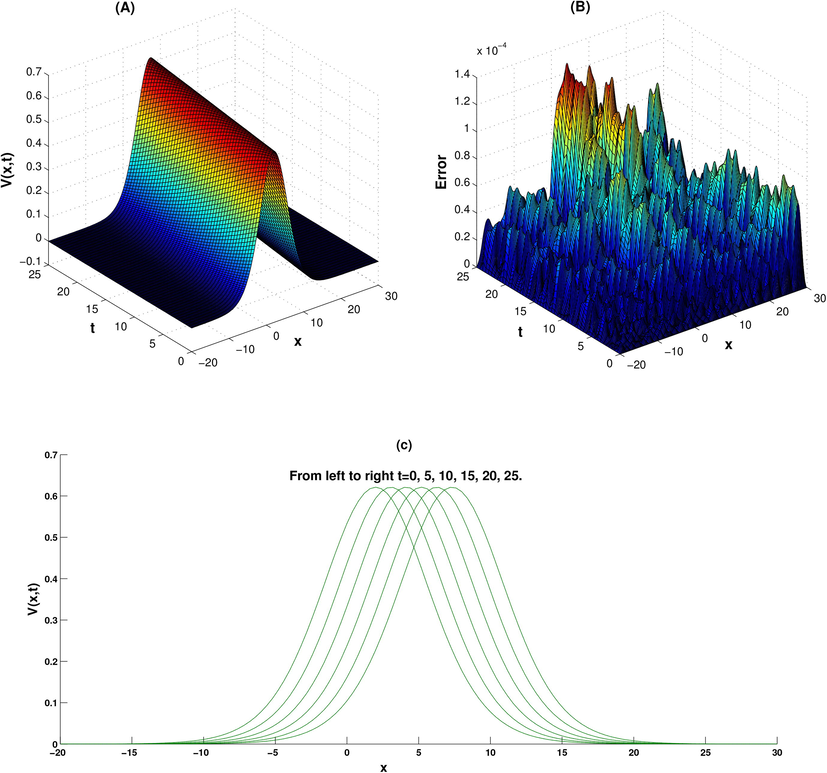
Graphs of approximation solutions (A) and errors (B), and plots of $V(x,t)$ at $t=0,5,10,15,20,25$ (C), using the RBF-FD method with $∊=2,h=1/10,n_s=50$ and $\tau =1/100$ for Example 1.

Export to PPT

This equation is the sum of two solitary waves that are located at $x_1=0$ and $x_2=20$. For $-50⩽x\le 100,0⩽t⩽50,\mu =\sqrt{16/105},{\rho }_i=(12-2i)/13,d_i={\rho }_i/\mu ,i=1,2\text{.}$ It is solved by using RBF-FD method with $\tau =0.01,h=0.2$ and $∊=1$. The propagating of both waves toward the right is shown in Fig. 2. Also, the two invariants $I_1$ and $I_2$ are preserved constant laws as it shown in the Table 5.

Close

Fig. 2

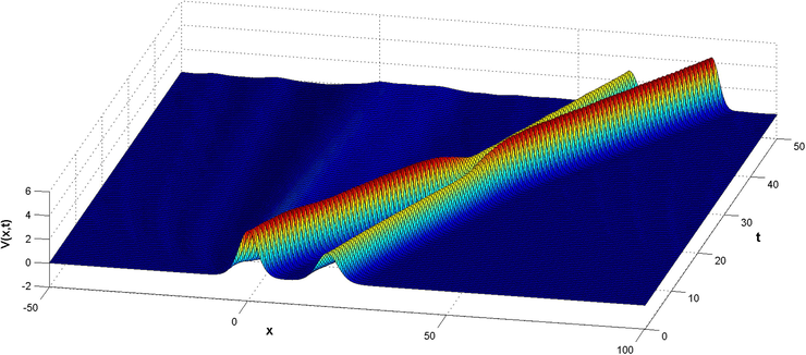
Graphs of approximation solutions using the RBF-FD method with $∊=2,h=1/10,n_s=50$ and $\tau =1/100$ for Example 2.

Export to PPT

This equation is the sum of three solitary waves that are located at $x_1=-20,x_2=0$ and $x_3=20$. For $-30⩽x⩽120,0⩽t⩽60,\mu =\sqrt{16/105},{\rho }_i=(12-2i)/13,d_i={\rho }_i/\mu ,i=1,2,3$,it is solved using RBF-FD method with $\tau =0.01,h=0.2,n_s=50$ and $∊=1$. The motion of three waves from the left to the right is shown in Fig. 3.

Close

Fig. 3

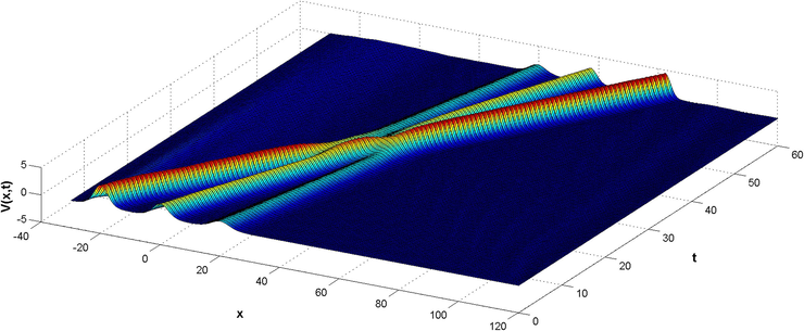
Graphs of approximation solutions using the RBF-FD method with $∊=2,h=1/10,n_s=50$ and $\tau =1/100$ for Example 3.

Export to PPT

This example also has been solved by RBF-FD method. The graphs of approximation solution and point wise error, and the interaction profile of single solitary wave with $\tau =0.001,h=0.1,\epsilon =2,n_s=50$ on region $(x,t)\in [-20,50]\times [0,60]$ has been shown in Fig. 4. In the Table 6, a comparison of the error norms $L_2$ and $L_{\infty }$, and invariants $I_1$ and $I_2$ between proposed method and RBFs method (Haq and Uddin, 2011) is reported. From this table it is clear that the presented method has a good agreement with the exact result and has a better accuracy than the RBF method (Haq and Uddin, 2011). Also, the respected changes of invariants $I_1$ and $I_2$ of RBF-FD method are approximately constant and acceptable. Furthermore, the condition number of the RBF-FD method is equal to $5.9063e+04$ and the RBF method (Haq and Uddin, 2011) is equal to $1.5063e+10$. Thus, the RBF-FD method is more well-conditioned than the RBF one. Therefore, these results verify an improvement of the RBF-FD method versus RBFs (Haq and Uddin, 2011) ones.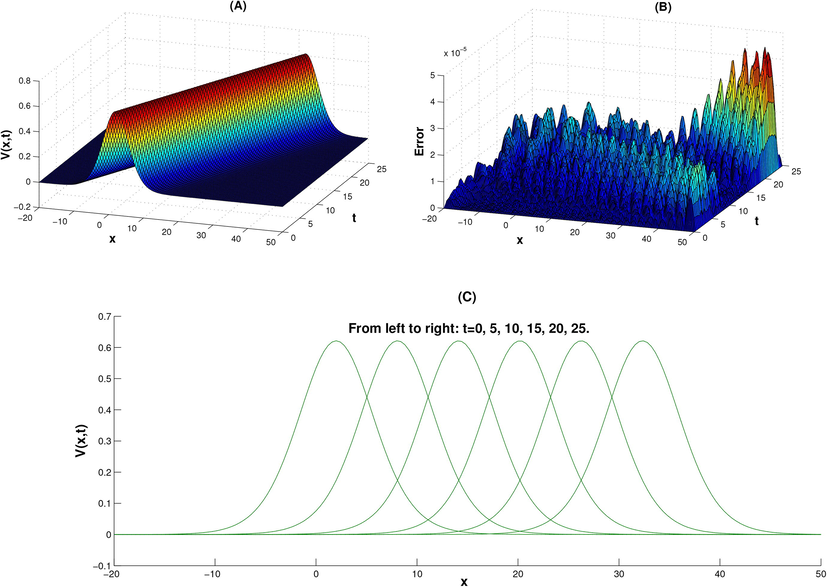

Close

Fig. 4

Graphs of approximation solutions (A) and errors (B), and plots of $V(x,t)$ at $t=0,5,10,15,20,25$ (C), using the RBF-FD method with $∊=2,h=1/10,n_s=50$ and $\tau =1/1000$ for Example 4.

Export to PPT

References

- Reduced differential transform method and its application on Kawahara equations. Thai J. Math.. 2012;11(1):199-216.
- [Google Scholar]
- Homotopy analysis method for the Kawahara equation. Nonlinear Anal.: Real World Appl.. 2010;11(1):307-312.
- Solitons, nonlinear evolution equations and inverse scattering. Vol vol. 149. Cambridge University Press; 1991.
- An efficient approximation to numerical solutions for the Kawahara equation via modified cubic B-Spline differential quadrature method. Mediterr. J. Math.. 2019;16(1):14.
- mixed algorithm for numerical computation of soliton solutions of the coupled KdV equation: finite difference method and differential quadrature method. Appl. Math. Comput.. 2019;360:42-57.
- A novel approach via mixed Crank-Nicolson scheme and differential quadrature method for numerical solutions of solitons of mKdV equation. Pramana-J. Phys.. 2019;92(6):84.
- An effective approach to numerical soliton solutions for the Schrödinger equation via modified cubic B-spline differential quadrature method. Chaos, Solitons Fractals. 2017;100:45-56.
- RBF-FD formulas and convergence properties. J. Comput. Phys.. 2010;229(22):8281-8295.
- Meshless method of lines for numerical solution of Kawahara type equations. Appl. Math.. 2011;2(05):608.
- The Korteweg-de Vries-Kawahara equation in a bounded domain and some numerical results. Appl. Math. Comput.. 2007;190(1):912-936.
- local meshless method for solving multi-dimensional Vlasov-Poisson and Vlasov-Poisson-Fokker-Planck systems arising in plasma physics. Eng. Comput.. 2017;33(4):961-981.
- numerical scheme based on radial basis function finite difference (RBF-FD) technique for solving the high-dimensional nonlinear Schrödinger equations using an explicit time discretization: Runge-Kutta method. Comput. Phys. Commun.. 2017;217:23-34.
- Soliton solutions for NLS equation using radial basis functions. Chaos, Solitons Fractals. 2009;42(2):1227-1233.
- Numerical methods for the solution of the third-and fifth-order dispersive Korteweg-de Vries equations. J. Comput. Appl. Math.. 1995;58(3):307-336.
- Approximation Methods with Matlab:(With CD-ROM).. Vol vol. 6. World Scientific Publishing Co Inc; 2007.
- Multi-symplectic Fourier pseudospectral method for the Kawahara equation. Commun. Comput. Phys.. 2014;16(1):35-55.
- RBFs approximation method for Kawahara equation. Eng. Anal. Boundary Elem.. 2011;35(3):575-580.
- Numerical simulation of solitary waves of Rosenau–KdV equation by Crank-Nicolson meshless spectral interpolation method. Eur. Phys. J. Plus. 2020;135(1):98.
- Travelling wave solutions to certain non-linear evolution equations. Int. J. Non-Linear Mech.. 1989;24(5):425-429.
- Numerical solutions of the Kawahara equation by the septic B-spline collocation method. Stat., Optim. Inf. Comput.. 2014;2(3):211-221.
- Application of optimal homotopy asymptotic method for the approximate solution of Kawahara equation. Appl. Math. Sci.. 2014;8(18):875-884.
- Crank-Nicolson-differential quadrature algorithms for the Kawahara equation. Chaos Solitons Fractals. 2009;42(1):65-73.
- Using radial basis function-generated finite differences (RBF-FD) to solve heat transfer equilibrium problems in domains with interfaces. Eng. Anal. Boundary Elem.. 2017;79:38-48.
- Interpolation of scattered data: distance matrices and conditionally positive definite functions. In: Approximation Theory and Spline Functions. Springer; 1984. p. :143-145.
- High accuracy cubic spline finite difference approximation for the solution of one-space dimensional non-linear wave equations. Appl. Math. Comput.. 2011;218(8):4234-4244.
- new high accuracy cubic spline method based on half-step discretization for the system of 1D non-linear wave equations. Eng. Comput.. 2019;36(3):930-957.
- meshless method for solving mKdV equation. Comput. Phys. Commun.. 2012;183(6):1259-1268.
- Solitary wave solution of the nonlinear KdV-Benjamin-Bona-Mahony-Burgers model via two meshless methods. Eur. Phys. J. Plus. 2019;134(7):367.
- Numerical investigation of the nonlinear modified anomalous diffusion process. Nonlinear Dyn.. 2019;97(4):2757-2775.
- Numerical methods based on radial basis function-generated finite difference (RBF-FD) for solution of GKdVB equation. Wave Motion. 2019;90:152-167.
- Solitary waves solutions of the MRLW equation using quintic B-splines. J. King Saud Univ.-Sci.. 2010;22(3):161-166.
- The evaluation of compound options based on RBF approximation methods. Eng. Anal. Boundary Elem.. 2015;58:112-118.
- Adaptive radial basis function methods for time dependent partial differential equations. Appl. Numer. Math.. 2005;54(1):79-94.
- Collocation method for Convection-Reaction-Diffusion equation. J. King Saud Univ.-Sci.. 2019;31(4):1115-1121.
- Shechter, G., 2004. Matlab package kdtree.
- New exact travelling wave solutions for the Kawahara and modified Kawahara equations. Chaos Solitons Fractals. 2004;19(1):147-150.
- The optimal homotopy-analysis method for Kawahara equation. Nonlinear Analysis: Real World Applications. 2011;12(3):1555-1561.
- Scattered node compact finite difference-type formulas generated from radial basis functions. J. Comput. Phys.. 2006;212(1):99-123.
- On a solution on non-linear time-evolution equation of fifth order. J. Phys. Soc. Jpn.. 1981;50(5):1421-1422.
- Periodic and solitary wave solutions of Kawahara and modified Kawahara equations by using Sine-Cosine method. Chaos, Solitons Fractals. 2008;37(4):1193-1197.