

Translate this page into:
Numerical simulation of two-dimensional modified Helmholtz problems for anisotropic functionally graded materials
⁎Corresponding author. mohivanazis@yahoo.co.id (Moh. Ivan Azis)
-
Received: ,
Accepted: ,
This article was originally published by Elsevier and was migrated to Scientific Scholar after the change of Publisher.
Abstract
The paper focuses on finding solutions to modified Helmholtz BVPs of anisotropic FGMs.
Abstract
In this paper we consider the modified Helmholtz type equation governing 2D-boundary value problems for anisotropic functionally graded materials (FGMs) with Dirichlet and Neumann boundary conditions. The persistently spatially changing diffusion and leakage factor coefficients involved in the governing equation indicate the inhomogeneity of the material under consideration. And the anisotropic diffusion coefficients indicate the material’s anisotropy. Some particular examples of problems are solved numerically using a boundary element method (BEM). The results show the accuracy and consistency of the numerical solutions, the effect of the coefficient values on the solutions, and the impact of the inhomogeneity and the isotropy of the materials to the solutions.
Keywords
Boundary element method
Modified Helmholtz problems
Anisotropic functionally graded media
65N38

1 Introduction
Authors commonly define an FGM as an inhomogeneous material having a specific property such as thermal conductivity, hardness, toughness, ductility, corrosion resistance, etc. that changes spatially in a continuous fashion. Nowadays FGM has become an important topic, and numerous studies on FGM for a variety of applications have been reported (see e.g. Bakhadda et al., 2018; Bounouara et al., 2016; Hedayatrasa et al., 2014; Karami et al., 2017; Karami et al., 2018a; Karami et al., 2018b; Karami et al., 2018c; Karami et al., 2019a; Karami et al., 2019b and Zemri et al., 2015).
The modified Helmholtz equation appears in many kind of applications such as neutron diffusion problems (Itagaki and Brebbia, 1993), advection-diffusion problems (Solekhudin and Ang, 2012), problems governed by Laplace type equation (Chen et al., 2002), Debye-Huckel theory and the linearized Poisson–Boltzmann problems (Kropinski and Quaife, 2011), steady-state groundwater flow (Gusyev and Haitjema, 2011) and unsteady heat conduction (Guo et al., 2013). So many works which are related to the modified Helmholtz equation and focusing on finding its numerical solutions have been done, yet most of the works are limited to the case of isotropic and/or homogeneous media. The works by Igarashi and Honma (1992), Itagaki and Brebbia (1993), Singh and Tanaka (2000), Chen et al. (2002), Cheng et al. (2006), Gusyev and Haitjema (2011), Kropinski and Quaife (2011), Guo et al. (2013), Nguyen et al. (2013) and Chen et al. (2014) are among the examples.
Apparently, BEM has been successfully used for solving many types of problems of either homogeneous or functionally graded (inhomogeneous), and either isotropic or anisotropic materials. Some works using BEM for homogeneous anisotropic media of 2D diffusion-convection and Helmholtz problems (e.g. Azis et al. (2018); Azis, 2019a) have been recently reported. And for inhomogeneous anisotropic media BEM also has been used to solve elasticity, scalar elliptic, Helmholtz, diffusion-convection and diffusion-convection–reaction problems (see e.g. Azis and Clements, 2014; Azis, 2019b; Azis, 2019c; Hamzah et al., 2019; Lanafie et al., 2019; Haddade et al., 2019; Azis et al., 2019; Hamzah et al., 2019).
This paper discusses derivation of a BEM for numerically solving 2D problems governed by the modified Helmholtz type equation for anisotropic FGMs of the form
For Eq. (1) to be an elliptic partial differential equation throughout , the matrix of coefficients is required to be a symmetric positive definite matrix. The coefficients and are also required to be twice differentiable functions.
Throughout the paper, the analysis used is purely mathematical; to develop a BEM for obtaining the numerical solution of problems governed by Eq. (1) is the main purpose. The analysis in general applies for anisotropic media, but it is equally applicable to isotropic materials as a special case occurring when and . Likewise, the analysis also applies especially for homogeneous materials, as a special case of FGMs, that occurs when and are constant. Therefore the main aim of this paper is to make the coverage of (1) wider as to cover the case of anisotropic FGMs as well as the special case of isotropic homogeneous materials which mostly had been worked on previously.
2 The boundary value problem
Referred to a Cartesian frame a solution to (1) is sought which is valid in a region in with boundary consisting of a number of piecewise continuous curves. On either or is specified, where
and is the normal vector pointing out on the boundary . A boundary integral equation will be sought, from which numerical values of the dependent variables and its derivatives may be obtained for all points in .
3 The boundary integral equation
The boundary integral equation is derived by transforming the variable coefficient Eq. (1) to a constant coefficient equation. We restrict the coefficients and to be of the form
Assume
Use of the identityallows Eq. (7) to be written in the form
So that if g satisfies
Moreover, substitution of (3) and (6) into (2) gives
Three possible multi parameter function satisfying (8) are for which for which and , and for which and . When the material under consideration is a layered material consisting of several layers where each layer is a specific type of material of specific constant coefficients and then the discrete variation of the constant coefficients from layer to layer may certainly accommodate the determination of a continuous variation of the variable coefficients and by interpolation, that is to determine the parameters of function .
An integral equation for (9) is
Eq. (14) provides a boundary integral equation which is the starting point of BEM construction for determining the numerical solutions of and its derivatives at all points of .
4 Numerical examples
To illustrate the use of BEM some examples of problems governed by (1) are considered. For a simplicity, the domain is taken to be a unit square for all problems (see Fig. 1). Hankel and the modified Bessel functions in (12) and (13) are approximated by their ascending series, and the integral in (14) is evaluated using Gaussian quadrature (see Abramowitz and Stegun, 1972). A number of 640 (constant) boundary elements of equal length, that is 160 elements on each side of the unit square domain, are used for the implementation of BEM.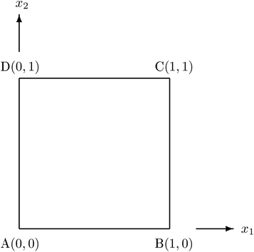
The domain .
4.1 Problems with analytical solutions
Some problems with analytical solutions will be considered. The aim is to evaluate the accuracy and efficiency of the numerical solutions. In addition to this, the impact of an increase of the coefficient on the accuracy, when appropriate, will also be investigated. For all test problems considered, the boundary conditions are
4.1.1 Example 1: anisotropic quadratically graded material
For one of the possible forms of satisfying (8) is the quadratic function that is when a quadratically graded material is under consideration. The constant coefficient is
We take several values of . The values of and corresponding maximum value of wave number and analytical solutions are shown in Table 1.
Analytical solution
6.71
13.41
5
26.83
20
53.66
Table 2 shows convergence of the numerical solutions and Table 3 indicates efficiency of the BEM. Specifically, the standard BEM only needs less than a minute time to obtain the solutions and its derivatives at 19 interior points. From this point forward, all the computation results are obtained using total number of 640 elements. Fig. 2 shows numerical absolute errors along the line for several values of . The errors are reasonably small occurring in the fourth decimal place. Fig. 2 also indicates that in general the errors increase as the value of gets larger.
Point
160 elements
320 elements
640 elements
Analytical
(0.1,0.5)
0.6154
0.6153
0.6150
0.6148
(0.3,0.5)
0.7993
0.7993
0.7991
0.7989
(0.5,0.5)
1.0561
1.0560
1.0558
1.0556
(0.7,0.5)
1.4140
1.4137
1.4135
1.4132
(0.9,0.5)
1.9131
1.9129
1.9125
1.9122
160 elements
320 elements
640 elements
4.59375
16.03125
59.65625
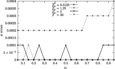
Numerical absolute errors along the line for Example 1.
4.1.2 Example 2: anisotropic exponentially graded material
When in Eq. (8), one of possible forms of is an exponential function of the form . The constant coefficients and k are taken to be
Table 4 shows several values of and corresponding maximum value of wave number and analytical solutions.
Analytical solution
0
0
0.5
0.31
1.84
0.91
3.14
4.66
7.12
19.66
131.59
Fig. 3 shows numerical absolute errors along the line for several different values of . The errors occur in the fourth decimal place, even with large values of . Again, the errors increase as the value of gets larger.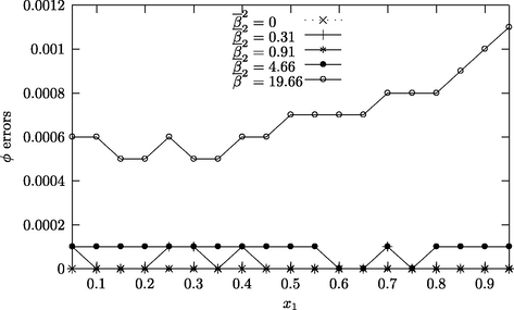
Numerical absolute errors along the line for Example 2.
4.1.3 Example 3: anisotropic trigonometrically graded material
Another possible forms of , when in Eq. (8), is a trigonometrical function where . Again, we take the constant coefficients and k
We intend to set the value of the coefficient in (9) to be negative, zero and positive, so as to consider three different types of Eq. (9). Therefore we choose thus . Table 5 shows the values of and corresponding analytical solutions.
Analytical solution
Fig. 4 shows numerical absolute errors along the line for three different values of . As for each represents a different type of Eq. (9), it is inappropriate to make a conclusion regarding the effect of values change on the errors.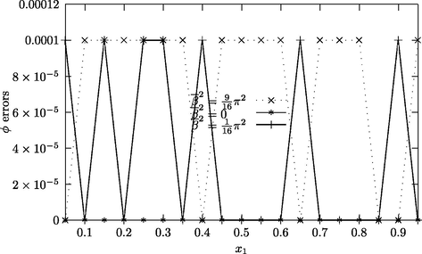
Numerical absolute errors along the line for Example 3.
4.2 Problems without any simple analytical solutions
Two problems will be considered. The boundary conditions are
4.2.1 Example 4
Now, the purpose is to show coherence between the flow vector and the scattering solutions inside the domain, and the impact of the inhomogeneity and the anisotropy of the material. The variable coefficients and for the governing Eq. (1) are
And we consider two cases regarding the anisotropy and inhomogeneity of the material as shown in Table 6.
Material
Isotropic homogeneous
4
Anisotropic inhomogeneous
Figs. 5 and 6 show a coherence between the flow vector and scattering solutions. This verifies that the developed FORTRAN code computes the flow vector correctly.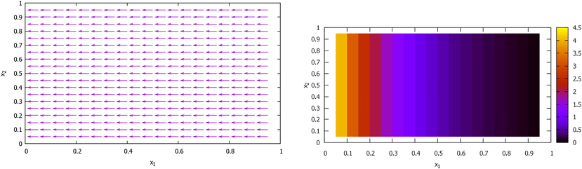
Flow and scattering solutions for Example 4 of the isotropic homogeneous material.
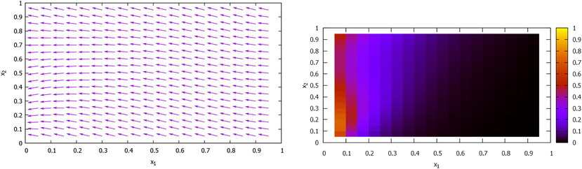
Flow and scattering solutions for Example 4 of the anisotropic inhomogeneous material.
4.2.2 Example 5
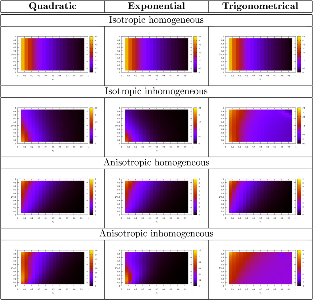
The aim is to see comparison of solutions for quadratically, exponentially and trigonometrically graded materials by keeping the parameters of the function , and the constant coefficients the same for all types of graded materials. Three types of material’s gradation and their forms of function are
The parameter chosen is and the values of constant matrix and the parameters associated with the anisotropy and inhomogeneity of the material are shown in Table 7.
Material
Isotropic homogeneous
Isotropic inhomogeneous
Anisotropic homogeneous
Anisotropic inhomogeneous
Table 8 shows a comparison of solutions inside the unit square domain for each combination of isotropy and homogeneity, and each type of types of material’s gradation. The results in Table 8 may be described as follows:
for each type of material, the impact of the anisotropy and inhomogeneity on the solutions is evident. This suggests that it is important to take into account the anisotropy as well as the inhomogeneity in application.
when the material is homogeneous (ie. so that ), either the material is isotropic or anisotropic, all the three types of material give identical solutions since the problems are identical.
contrarily, when the material is inhomogeneous (ie. ) the scattering solutions of the three types of material’s gradation are different. This is due to that the problems are not identical (the value k in Eqs. (8) and (9) is different) for each type of material’s gradation.
 |
5 Conclusion
It is possible to find numerical solutions of problems governed by an equation of variable coefficients such as the modified Helmholtz type Eq. (1) by using a standard BEM. Being adopted in this work, transformation of the variable coefficient equation into a constant coefficient equation is among way to derive a boundary integral equation. A BEM may then be constructed from the boundary integral equation. The standard BEM provides an ease of implementation, timeless computation and accurate solutions.
Modeling physical application for an anisotropic FGM always involves a variable coefficients governing equation such as (1). In this paper, quadratically, exponentially and trigonometrically graded materials are considered as the FGMs.
In addition to its accuracy, the BEM has also been working properly. This is indicated by the consistency between the flow vectors and scattering solutions. Moreover, it is also observed that the anisotropy and inhomogeneity of the material effect the results. This suggests both anisotropy and inhomogeneity should be taken into account in applications.
Acknowledgements
This work was supported by the Hasanuddin University, the Ministry of Education and Culture, and the Ministry of Finance of the Republic of Indonesia.
References
- Handbook of Mathematical Functions: With Formulas, Graphs and Mathematical Tables. Washington: Dover Publications; 1972.
- Fundamental solutions to two types of 2D boundary value problems of anisotropic materials. Far East J. Math. Sci.. 2017;101(11):2405-2420.
- [Google Scholar]
- Numerical solutions for the Helmholtz boundary value problems of anisotropic homogeneous media. J. Comput. Phys.. 2019;381:42-51.
- [Google Scholar]
- Standard-BEM solutions to two types of anisotropic-diffusion convection reaction equations with variable coefficients. Eng. Anal. Boundary Elem.. 2019;105:87-93.
- [Google Scholar]
- Numerical solutions to a class of scalar elliptic BVPs for anisotropic exponentially graded media. J. Phys: Conf. Ser.. 2019;1218:012001
- [Google Scholar]
- A boundary element method for transient heat conduction problem of non homogeneous anisotropic materials. Far East J. Math. Sci.. 2014;89(1):51-67.
- [Google Scholar]
- On some examples of pollutant transport problems solved numerically using the boundary element method. J. Phys: Conf. Ser.. 2018;979(1)
- [Google Scholar]
- BEM solutions to BVPs governed by the anisotropic modified Helmholtz equation for quadratically graded media. IOP Conf. Ser.: Earth Environ. Sci.. 2019;279:012010
- [Google Scholar]
- Dynamic and bending analysis of carbon nanotube-reinforced composite plates with elastic foundation. Wind Struct., Int. J.. 2018;27(5):311-324.
- [Google Scholar]
- A nonlocal zeroth-order shear deformation theory for free vibration of functionally graded nanoscale plates resting on elastic foundation. Steel Compos. Struct.. 2016;20(2):227-249.
- [Google Scholar]
- Dual boundary element analysis of oblique incident wave passing a thin submerged breakwater. Eng. Anal. Boundary Elem.. 2002;26:917-928.
- [Google Scholar]
- Singular boundary method for modified Helmholtz equations. Eng. Anal. Boundary Elem.. 2014;44:112-119.
- [Google Scholar]
- An adaptive fast solver for the modified Helmholtz equation in two dimensions. J. Comput. Phys.. 2006;211:616-637.
- [Google Scholar]
- Three-dimensional transient heat conduction analysis by Laplace transformation and multiple reciprocity boundary face method. Eng. Anal. Boundary Elem.. 2013;37:15-22.
- [Google Scholar]
- An exact solution for a constant-strength line-sink satisfying the modified Helmholtz equation for groundwater flow. Adv. Water Resour.. 2011;34:519-525.
- [Google Scholar]
- Numerical solutions to a class of scalar elliptic BVPs for anisotropic quadratically graded media. IOP Conf. Ser.: Earth Environ. Sci.. 2019;279:012007.
- [Google Scholar]
- On some examples of BEM solution to elasticity problems of isotropic functionally graded materials. IOP Conf. Ser.: Mater. Sci. Eng.. 2019;619:012018
- [Google Scholar]
- Numerical solutions to anisotropic BVPs for quadratically graded media governed by a Helmholtz equation. IOP Conf. Ser.: Mater. Sci. Eng.. 2019;619:012060
- [Google Scholar]
- Numerical modeling of wave propagation in functionally graded materials using time-domain spectral Chebyshev elements. J. Comput. Phys.. 2014;258:381-404.
- [Google Scholar]
- On axially and helically symmetric fundamental solutions to modified Helmholtz-type equations. Appl. Math. Model.. 1992;16:314-319.
- [Google Scholar]
- Multiple reciprocity boundary element formulation for one-group fission neutron source iteration problems. Eng. Anal. Boundary Elem.. 1993;11:39-45.
- [Google Scholar]
- Effects of triaxial magnetic field on the anisotropic nanoplates. Steel Compos. Struct.. 2017;25(3):361-374.
- [Google Scholar]
- Nonlocal strain gradient 3D elasticity theory for anisotropic spherical nanoparticles. Steel Compos. Struct.. 2018;27(2):201-216.
- [Google Scholar]
- Variational approach for wave dispersion in anisotropic doubly-curved nanoshells based on a new nonlocal strain gradient higher order shell theory. Thin-Walled Struct.. 2018;129:251-264.
- [Google Scholar]
- Galerkin’s approach for buckling analysis of functionally graded anisotropic nanoplates/different boundary conditions. Eng. Comput. 2018 In press
- [Google Scholar]
- On exact wave propagation analysis of triclinic material using three-dimensional bi-Helmholtz gradient plate model. Struct. Eng. Mech.. 2019;69(5):487-497.
- [Google Scholar]
- Resonance behavior of functionally graded polymer composite nanoplates reinforced with graphene nanoplatelets. Int. J. Mech. Sci.. 2019;156:94-105.
- [Google Scholar]
- Fast integral equation methods for the modified Helmholtz equation. J. Comput. Phys.. 2011;230:425-434.
- [Google Scholar]
- Numerical solutions to BVPs governed by the anisotropic modified Helmholtz equation for trigonometrically graded media. IOP Conf. Ser.: Mater. Sci. Eng.. 2019;619:012058.
- [Google Scholar]
- Some remarks on a modified Helmholtz equation with inhomogeneous source. Appl. Math. Model.. 2013;37:793-814.
- [Google Scholar]
- On exponential variable transformation based boundary element formulation for advection–diffusion problems. Eng. Anal. Boundary Elem.. 2000;24:225-235.
- [Google Scholar]
- A DRBEM with a predictor-corrector scheme for steady infiltration from periodic channels with root-water uptake. Eng. Anal. Boundary Elem.. 2012;36:1199-1204.
- [Google Scholar]
- A mechanical response of functionally graded nanoscale beam: an assessment of a refined nonlocal shear deformation theory beam theory. Struct. Eng. Mech.. 2015;54(4):693-710.
- [Google Scholar]


