

Translate this page into:
Numerical simulation of the transition of a Newtonian fluid to a viscoplastic state in a turbulent flow
⁎Corresponding author. uzak.zh@mail.ru (Uzak K. Zhapbasbayev),
-
Received: ,
Accepted: ,
This article was originally published by Elsevier and was migrated to Scientific Scholar after the change of Publisher.
Peer review under responsibility of King Saud University.
Abstract
The non-isothermal turbulent flow and transition to a viscoplastic state of high-viscosity oil with physical and chemical properties depending on fluid temperature is numerically studied. The turbulence of fluid flow in a pipe is described using the Reynolds stress, Reynolds algebraic stress, and two-parameter isotropic models. The simulations show the boundaries of the region of the manifestation of Newtonian behavior and fluid transition to a viscoplastic state. The Reynolds stress model and the algebraic Reynolds stress model show significant anisotropy in the velocity fluctuation profiles of Newtonian and non-Newtonian fluids. The shift of the locus of maximal magnitudes of turbulent pulsations, Reynolds stress, and turbulent kinetic energy towards a flow core region is observed. The height of the zone with a completely stopped fluid is predicted and determined numerically. The appearance of a stagnation zone near the wall causes a significant decrease in wall friction and heat transfer due to a decrease in the environment temperature.
Keywords
High-viscosity oil
Non-isothermal flow
Bingham-Schwedoff model
Turbulence
Heat transfer
Reynolds stress model

1 Introduction
Turbulent flows of waxy crude oil (WCO) with heat transfer with the environment occur in the main oil pipelines. The WCO flow can change from Newtonian state to viscoplastic one when environment temperature is cooled (Chhabra and Richardson, 2011; Souas et al., 2021; Zhumagulov et al., 2002). The material properties of such liquids have a strong nonlinear temperature dependence due to the presence of asphaltenes, paraffins, and resins (Aiyejina et al., 2011; Li et al., 2015). The appearance of yield stress causes the emergence of a “stagnant zone” formation in a near-wall zone, where flow rate fully stops (de Oliveira et al., 2010; Li et al., 2015). Therefore, transportation of high-viscosity oil through pipelines is complicated (Aiyejina et al., 2011; Li et al., 2015). Waxy crude oils at temperatures (T 298 K) are Newtonian fluids (NF). The viscoplastic behavior of a fluid appears by fluid temperature cooling (Aiyejina et al., 2011; Dai, 2019; Bekibayev et al., 2021, 2022; Zhapbasbayev et al., 2021).
Turbulent mean and fluctuational flow structure of a non-Newtonian fluid (NNF) often studied without heat transfer (Cruz and Pinho, 2003; Gavrilov and Rudyak, 2016b; Iaccarino et al., 2010; Malin, 1997). The experimental studies of such flows are very limited due to the complexity of the measurement methods (Escudier et al., 2009; Peixinho et al., 2005). The laser Doppler anemometry is used for measurements of a viscoelastic shear-thinning fluid (Escudier et al., 2009). The experiments were performed in a duct for a fully-developed flow. Three components of turbulent fluctuations and Reynolds shear stress were measured.
An alternative to this is to conduct mathematical modeling of non-Newtonian fluids. The turbulent flows of such fluids are usually modeled using the Reynolds-averaged Navier-Stokes equations (RANS) approach (Durbin and Pettersson Reif, 2011). In these works, turbulence models of various levels are used: k−ε (Cruz and Pinho, 2003; Malin, 1997), v2–f (Iaccarino et al., 2010). The difficulty arising in the mathematical modeling of such flows is that applied turbulence models are difficult to verify using known experimental benchmarks. The theoretical formula of the wall friction coefficient of turbulent Bingham–Schwedoff (BS) fluids is developed in (Anbarlooei et al., 2017).
Direct numerical simulation (DNS) and large eddy simulation (LES) are the main powerful methods for study of NNF. LES (Gnambode et al., 2015) and DNS (Gavrilov and Rudyak, 2016a; Rudman and Blackburn, 2006; Singh et al., 2017) works have been performed to investigate the turbulent power-law and viscoplastic and pseudoplastic non-Newtonian fluids. The results of average and fluctuational longitudinal and transverse velocities, wall friction, and the turbulent kinetic energy at Reynolds numbers, Re, from 5000 to 20,000 were obtained. Note that LES and DNS (Gavrilov and Rudyak, 2016a; Gnambode et al., 2015) only dealt with Buckley-Herschel fluids, and only recent paper (Singh et al., 2017) presents DNS prediction data for fluids with yield stress. A few papers concerned the study of heat transfer in turbulent NNF (Masoudian et al., 2016; Masoumi et al., 2019; Yigit et al., 2020). Turbulent flow studies with a viscoelastic flow of a polymer were investigated (Masoudian et al., 2016; Yigit et al., 2020). The DNS study of velocity and temperature spectra in Rayleigh-Bénard convection was performed in the paper (Yigit et al., 2020). The authors showed that thermal convection weakens with growth of the Rayleigh number. Numerical study of natural convection of Bingham–Schwedoff (BS) fluid between horizontal concentric cylinders was carried out in the paper (Masoumi et al., 2019).
The aim of this paper is numerically simulation of turbulent flow structure and heat transfer by transition of incompressible Newtonian fluid (WCO) to viscoplastic NNF in a pipe. This paper is a continuation of our recent work (Pakhomov and Zhapbasbayev, 2021). The authors studied transition of Newtonian fluid to viscoplastic state when cooling of nonisothermal turbulent flow in tube. The fluid flow turbulence is predicted by two-parameter k– model (Hwang and Lin, 1998). The papers (Gnambode et al., 2015) and DNS (Gavrilov and Rudyak, 2016a; Rudman and Blackburn, 2006; Singh et al., 2017) show that the anisotropy of velocity fluctuations is noticeably higher than that of a Newtonian fluid. Therefore, the use of isotropic turbulence models in the description of such flows is significantly limited by only obtaining results of the mean flow, while predictions of the turbulent characteristics using this approach have led to significant errors.
In this work, the RSM (Manceau and Hanjalic, 2002) and the explicit algebraic Reynolds stress model (ARSM) (Rokni, 2000; Speziale and Xu, 1996) were used to describe the anisotropy property. The following are the research results of turbulent flow and heat transfer of WCO in a pipe using the RSM and the ARSM.
2 Mathematical model
2.1 Bingham-Schwedoff rheology model
Waxy crude oil rheology can be modeled as the generalized Newtonian fluids (Vinay et al., 2005; Salehi-Shabestari et al., 2016). The effective (apparent) viscosity of a BS fluid is defined using a rheology model (Barnes, 1999; Beverly and Tanner, 1992; Bingham, 1922). The Bingham-Schwedoff model is the simplest model of viscoplastic non-Newtonian fluids (Barnes, 1999; Bingham, 1922):
The singularity of a numerical solution of the Eq. (1) is appeared in zones at τ < τ0. The singular property of the effective viscosity can be solved by improving the original rheological model (Barnes, 1999). Effective viscosity can be represented as a smooth function using the approach (Papanastasiou, 1987):
2.2 The set of governing equations for a non-Newtonian turbulent fluid
The system of stationary RANS equations for the flow and heat transfer of an incompressible fluid has the form
Here, S is averaged strain rate tensor, is modulus of averaged strain rate tensor. The turbulent characteristics and was written according to Boussinesq hypothesis. The expression in equation (4) is found according to representation (Gavrilov and Rudyak, 2016b). The last term in equation (5) takes into account the dissipation of kinetic energy and has the form (Vinay et al., 2005). In the recent paper (Pakhomov and Zhapbasbayev, 2021) the system of equations (3)–(5) was solved jointly with k– model (Hwang and Lin, 1998).
The elliptical relaxation RSM (Manceau and Hanjalic, 2002) considers anisotropy of complex turbulent flows and is computationally more difficult than ARSM. These models give better predictable results than the k-
turbulence isotropic model. The ARSM from (Rokni, 2000) is a version of the well-known explicit Reynolds algebraic stress model (Speziale and Xu, 1996). The Reynolds stress components are derived from a system of partial differential equations, and the system of basic equations of the second-moment closure model of (Manceau and Hanjalic, 2002) is given:
Here, Pij is the intensity of the energy transfer from the average velocity to the pulsating one; P2 = 0.5Pkk, TT is the turbulent time macroscale; ϕ is the redistribution term (Manceau and Hanjalic, 2002), ε is the dissipation rate.
2.3 Boundary conditions
All boundary conditions for a non-isothermal flow are given in details (Pakhomov and Zhapbasbayev, 2021). No-slip conditions are set on the wall surface for fluid velocity. The heat transfer coefficient from fluid flow (WCO) to cold soil through pipe surface is determined by the formula (Zhapbasbayev et al., 2021). The symmetry conditions are set on the pipe axis. The uniform distributions of velocity and temperature are set over the cross-section of pipe in inlet section. At the outlet edge, gradients of all flow and heat transfer parameters in axial direction.
3 Numerical realization
The flow sketch is shown in the Fig. 1. Numerical predictions are carried out using the “in-house” code. The system of equations (3)–(7) is solved numerically using the QUICK scheme and the SIMPLEC algorithm. The simulations use a non-uniform mesh with refinement close to all walls. The cell closest to the wall is located at y+ = yu*/νW = 0.4, where y = R – r is distance from the wall, R is pipe radius, u* is friction velocity of a Newtonian fluid in the inlet pipe and νW is kinematic viscosity of a fluid at wall condition. The residual error for the continuity equation, momentum equations, and RSM model is 10−5 and for the energy equation the error is 10−7.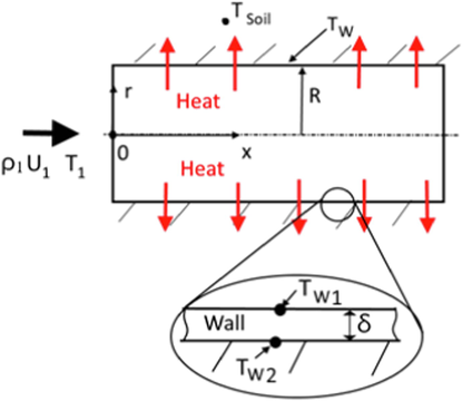
Flow configuration scheme.
The grid convergence test (GCT) is performed on the grids: 500 × 40 (coarse), 1000 × 80 (medium) and 1500 × 120 (fine) (see Fig. 2). The GCT results are presented for the RSM (Manceau and Hanjalic, 2002) (see Fig. 2a) and the ARSM (Rokni, 2000) (see Fig. 2b). The GCT for the k–
model was carried out in (Hwang and Lin, 1998). The Reynolds and Prandtl numbers of the flow are Re = U1D/νW1 = 0.82 × 10⁴ and Pr = µW1CP1/λ1 = 42.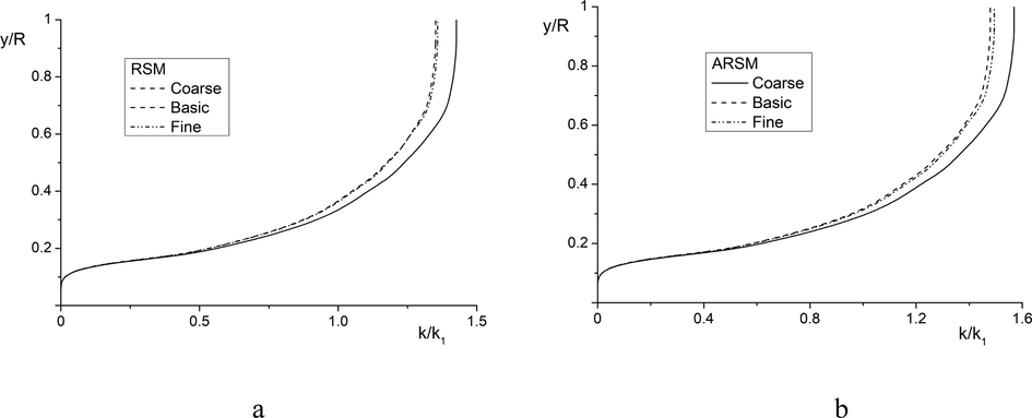
The grid convergence test of ''in-house'' code for the RSM (a) and the ARSM (b). L = 2 m, Re = 8200, U1 = 0.2 m/s, T1 = 298 K, TW = 273 K.
4 Results and discussion
4.1 Isothermal flow in a pipe
At the first stage, the comparisons with data of DNS predictions for the turbulent flow of Newtonian fluid in pipe were performed. DNS simulations (Singh et al., 2017) on the transverse distributions of axial and radial velocity fluctuations for Newtonian turbulent fluid were used. These results are given in Fig. 3. The maximum differences in the intensity of the axial pulsations of the Newtonian fluid velocity do not exceed 10% when predicted using the RSM model (see Fig. 3a). The largest discrepancy between the data of our numerical RANS simulations and DNS data (Singh et al., 2017) does not exceed 15% and is observed for radial pulsations (see Fig. 3b) at y+ ≈ 80.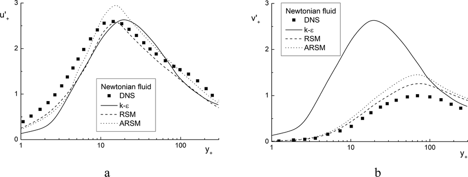
Radial profiles of axial (a) and radial (b) velocities pulsations of a Newtonian fluid. Solid symbols are the DNS results (Singh et al., 2017) and lines are authors’ RANS predictions. Solid lines are the k–
model (Hwang and Lin, 1998), dashed curves are the RSM (Manceau and Hanjalic, 2002) and dotted lines are the ARSM (Rokni, 2000). Re = 1.3 × 10⁴, Reτ = 323.
Fig. 4 shows the profiles of (a) axial and (b) radial velocity fluctuations of the Bingham–Schwedoff fluid over the pipe section in the wall units y+. The dots are the DNS data (Singh et al., 2017), the lines are the authors’ RANS predictions. The solid lines are the k–
model (Hwang and Lin, 1998), the dashed lines are the RSM model (Manceau and Hanjalic, 2002) and the dotted lines are the full explicit ARSM (Rokni, 2000). In the calculations of the k–
model (Hwang and Lin, 1998), the individual components of the Reynolds stresses are determined in the framework of the isotropic representation:
. Satisfactory agreement between our simulations and the data of DNS predictions is obtained only when using the RSM approach.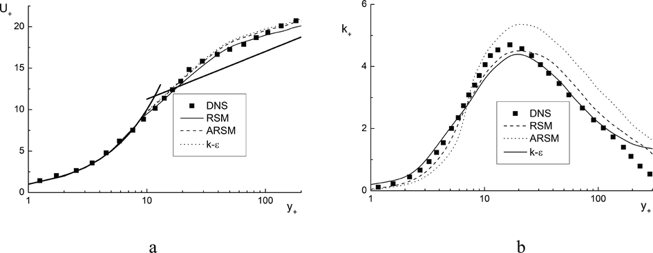
Profiles of average axial velocity (a) and turbulent kinetic energy (b) of a NNF. Solid symbols are DNS results (Singh et al., 2017) and lines are authors’ RANS predictions. Solid lines are the k–
model (Hwang and Lin, 1998), dashed curves are the RSM (Manceau and Hanjalic, 2002) and dotted lines are the ARSM (Rokni, 2000). Re = 1.3 × 10⁴, Reτ = 323, τ0/τW = 1.2.
The significant anisotropy of profiles velocity pulsations of a non-Newtonian fluid is obtained in predictions using RSM and ARSM, which is consistent with the data of (Singh et al., 2017) (see Table 1). The positions of the maxima in the distributions of axial and radial pulsations are in satisfactory agreement with the positions of the maxima for DNS (Singh et al., 2017). An exception is the distribution of radial fluctuations
predicted using the isotropic k–
model (Hwang and Lin, 1998) (see Table 2). The radial velocity fluctuations are significantly less than the intensity of axial fluctuations. The (Hwang and Lin, 1998) model describes well distribution of axial pulsation component along pipe radius (difference does not exceed 15%). In this case, there is a significant excess of radial fluctuations in comparison with the data [22] and our calculations using anisotropic turbulence models (Manceau and Hanjalic, 2002; Rokni, 2000) (up to 3 times).
Reference
y+ = 30
y+ = 50
y+ = 100
y+ = 200
DNS (Singh et al., 2017)
3.6
2.4
1.8
1.5
RSM (Manceau and Hanjalic, 2002)
2.8
2.1
1.6
1.35
ARSM (Rokni, 2000)
2.5
1.7
1.3
1.1
Reference
DNS (Singh et al., 2017)
16
85
RSM (Manceau and Hanjalic, 2002)
17.5
90
ARSM (Rokni, 2000)
17
75
k–
(Hwang and Lin, 1998)
20
20
The comparison of the DNS data (Singh et al., 2017) and our calculations of the axial velocity and kinetic energy of turbulence (KET) in wall units for the BS fluid are presented in Fig. 4. Here dots in Fig. 4b are the DNS data (Singh et al., 2017), curves are authors’ RANS calculation by using k– (Hwang and Lin, 1998), the RSM (Manceau and Hanjalic, 2002) and the ARSM (Rokni, 2000) turbulence models. Fig. 4a shows the velocity profiles U+ for NNF. Difference between the three turbulence models is insignificant in the regions (y+ < 5 and (5 < y+ < 30). These results quantitative agree with the DNS data (Singh et al., 2017) (see Fig. 4a). Yield stress has practically no effect within the viscous sublayer and the differences between the various models are minimal. It qualitatively agrees with the conclusions of (Wilson and Thomas, 1985). For all three models, the difference is no more than 15% and the velocity profile is similar for a NF. Our RANS predictions and DNS at 30 < y+ < 200 differ by up to 15%.
4.2 Turbulent non-isothermal flow structure
The distribution of the action zone of yield stress τ0/τNF = 10 along the axial coordinate depending on the ambient soil temperature is shown in Fig. 5. The zone height of yield stress τ0/τNF = 10 increases gradually along the streamwise coordinate. It tends to the coordinate y/R ≈ 0.6 at x/D = 40 (x = 8 m) for temperature TS = 273 K and y/R ≈ 0.06 for temperature TS = 293 K.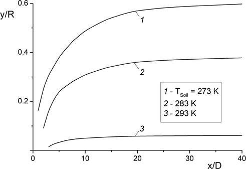
Evolution of radial coordinates of yield stress values presence τ0/τNF = 10 along the pipe length. Re = 8200, T1 = 298 K.
The effect of ambient soil temperature on the radial profiles of yield stress y/R is shown in Fig. 6. The viscoplastic non-Newtonian behavior of WCO is clearly shown at TS = 273 K. In this case, the fluid with the manifestation of NNF properties occupies the most part of pipe cross-section (y/R ≤ 0.75). The yield stress value exceeds the stresses in a turbulent Newtonian fluid flow by several orders of magnitude. The magnitude of yield shear stress is minimal at TS = 293 K. The non-Newtonian behavior of waxy crude oil appears only in the pipe near-wall part (y/R ≤ 0.2).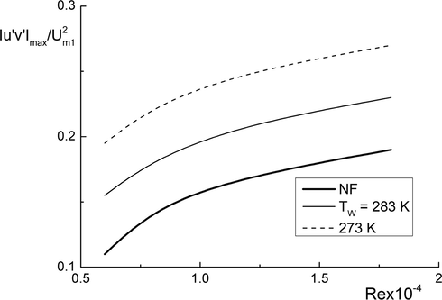
Effect of Reynolds number on distributions of maximal values of the Reynolds stress. x/D = 20, T1 = 298 K, TSoil = 273 K.
4.3 Wall friction and heat transfer
In Fig. 7 distributions of wall friction and Nusselt numbers are represented at x/D = 10. Here wall friction coefficient is
and the Nusselt number is Nu = hD/λW, heat transfer coefficient is h. Abbreviation FD is a fully developed Newtonian fluid and subscript W is a wall. The results are given in Fig. 7 are conducted for the developing flow of Newtonian waxy crude oil (NF line), and for the hydrodynamically fully developed Newtonian waxy crude oil (FD line). Therefore, the magnitude of heat transfer in the developing flow is higher than in the developed flow under all other conditions being equal. The coefficients of friction and heat transfer increase with an increase in the Reynolds number at the pipe inlet (see Fig. 7). It can be seen that the decrease in surrounding soil temperature causes a more rapid manifestation of the non-Newtonian properties of a Bingham-Schwedoff fluid and this confirms the conclusions from our previous predicted results. This leads to an increase in resistance (Fig. 7a) and a weakening of heat transfer (see Fig. 7b) of turbulent flow in pipe. Fluid velocity increase leads to a slow cooling of the turbulent flow, as well as an increase in the pipe length, where the Newtonian property of the fluid preserved.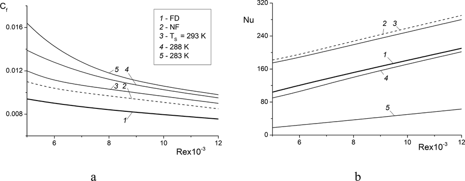
Effect of Reynolds numbers on wall friction and Nusselt number at x/D = 10.
The normalized distributions of wall friction Cf/Cf,fd (a) and heat transfer Nu/Nufd (b) on the wall during the turbulent fluid flow along streamwise coordinate are given in Fig. 8. A decrease in the environment temperature leads to a significant reduction in wall friction Cf and heat transfer Nu. Close to the wall, yield stress and a fluid stagnation zone appear (a medium behaves like a solid). The magnitudes of Cf, Nu are equal to zero in this region. In the case of the manifestation of the yield stress in the near-wall region of the pipe, heat transfer is possible only due to thermal conductivity. It qualitatively agrees with the conclusions of (Aljerf, 2016; Aljerf and Al Masri, 2018).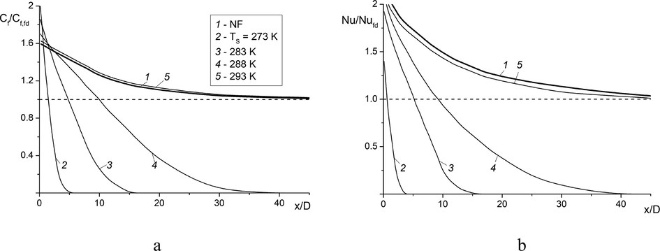
Influence of soil temperature TS on wall friction (a) and transfer (b) distributions of WCO along pipe length. Re = 8200, T1 = 298 K.
5 Conclusion
A numerical RANS predictions of heat transfer of Bingham–Schwedoff fluid has been carried out. Fluid turbulence is described by the Reynolds stress model. A comparison is carried out with the DNS data predictions of a Bingham–Schwedoff isothermal turbulent fluid. The RSM agrees better with the DNS data on turbulent characteristics for an isothermal non-Newtonian Bingham–Schwedoff fluid than the ARSM and the k– model.
Satisfactory agreement between our simulations and the DNS is obtained only using the RSM approach. The significant anisotropy of the profiles of velocity pulsations of a non-Newtonian fluid is obtained in predictions using the RSM and the ARSM. The anisotropy coefficient of pulsation velocities reaches ≈ 5.3. The shift of the locus of maximal values of turbulent pulsations, Reynolds stress, and turbulent kinetic energy towards the flow core is observed. In calculations, region of transition of Newtonian fluid to viscoplastic state is determined. An increase in fluid velocity leads to an increase in the pipe length, where Newtonian properties of fluid are preserved due to slower cooling of turbulent fluid flow.
The appearance of a non-Newtonian fluid property leads to an increase in resistance and a weakening of the heat transfer of a turbulent flow in the pipe. A decrease in surrounding environment temperature causes a significant decrease in the coefficient of wall friction and heat transfer due to the appearance of yield stress. The height of a stagnation zone of the fluid flow is numerically predicted. Close to the wall, yield stress and a fluid stagnation zone appear (a medium behaves like a solid). The magnitudes of Cf, Nu are equal to zero in this region. Heat transfer in the case of manifestation of yield stress in near-wall region of pipe is possible only due to thermal conductivity.
Acknowledgements
This work supported by the Science Committee of the Ministry of Science and Higher Education of the Republic of Kazakhstan (Grant number AP14869322 for 2022-2024).
Declaration of Competing Interest
The authors declare that they have no known competing financial interests or personal relationships that could have appeared to influence the work reported in this paper.
References
- Wax formation in oil-pipelines: a critical review. Int. J. Multiph. Flow. 2011;37:671-694.
- [Google Scholar]
- Reduction of gas emission resulting from thermal ceramic manufacturing processes through development of industrial conditions. Sci. J. King Faisal Univ.. 2016;17(1):1-10.
- [Google Scholar]
- Flame propagation model and combustion phenomena: observations, characteristics, investigations, technical indicators, and mechanisms. J. Energy Conserv.. 2018;1(1):31-40.
- [Google Scholar]
- Phenomenological friction equation for turbulent flow of Bingham fluids. Phys. Rev. E. 2017;96:023107
- [Google Scholar]
- The yield stress−a review or ‘παντα ρει’−everything flows? J. Nonnewton. Fluid Mech.. 1999;81:133-178.
- [Google Scholar]
- Simulation of oil pipeline shutdown and restart modes. Complex Use Min. Resour.. 2021;316:15-23.
- [Google Scholar]
- Optimal regimes of heavy oil ransportation through a heated pipeline. J. Process Control. 2022;115:27-35.
- [Google Scholar]
- Numerical analysis of three-dimensional Bingham plastic flow. J. Nonnewton. Fluid Mech.. 1992;42:85-115.
- [Google Scholar]
- Fluidity and plasticity. New York, U.S.A.: McGraw-Hill; 1922.
- Non-Newtonian Flow and Applied Rheology: Engineering Applications. Oxford, U.K.: Butterworth-Heinemann; 2011.
- Turbulent pipe flow predictions with a low Reynolds number k-e model for drag reducing fluids. J. Nonnewton. Fluid Mech.. 2003;114:109-148.
- [Google Scholar]
- Analysis on influencing factors of buried hot oil pipeline. Case Stud. Therm. Eng.. 2019;16:100558
- [Google Scholar]
- Numerical simulation of the start-up of Bingham fluid flows in pipelines. J. Non-Newt. Fluid Mech.. 2010;165:1114-1128.
- [Google Scholar]
- Reynolds Averaged Navier-Stokes Equations. Statistical Theory and Modeling for Turbulent Flows, 45–56. 2nd Edition, Chapter 3. Chichester, U.K.: John Wiley & Sons, Ltd; 2011.
- Turbulent flow of viscoelastic shear-thinning liquids through a rectangular duct: Quantification of turbulence anisotropy. J. Nonnewton. Fluid Mech.. 2009;160:2-10.
- [Google Scholar]
- Large-eddy simulation of turbulent pipe flow of power-law fluids. Int. J. Heat Fluid Flow. 2015;54:196-210.
- [Google Scholar]
- Direct numerical simulation of the turbulent flows of power-law fluids in a circular pipe. Thermophys. Aeromech.. 2016;23:473-486.
- [Google Scholar]
- Reynolds-averaged modeling of turbulent flows of power-law fluids. J. Nonnewton. Fluid Mech.. 2016;227:45-55.
- [Google Scholar]
- Improved low-Reynolds-number k– model based on direct simulation data. AIAA J.. 1998;36:38-43.
- [Google Scholar]
- Reynolds-averaged modeling of polymer drag reduction in turbulent flows. J. Nonnewton. Fluid Mech.. 2010;165:376-384.
- [Google Scholar]
- The influence of the heating temperature on the yield stress and pour point of waxy crude oils. J. Pet. Sci. Eng.. 2015;135:476-483.
- [Google Scholar]
- The turbulent flow of Bingham plastic fluids in smooth circular tubes. Int. Comm. Heat Mass Transfer. 1997;24:793-804.
- [Google Scholar]
- Elliptic blending model: a new near-wall Reynolds-stress turbulence closure. Phys. Fluids. 2002;14:744-754.
- [Google Scholar]
- A RANS model for heat transfer reduction in viscoelastic turbulent flow. Int. J. Heat Mass Transf.. 2016;100:332-346.
- [Google Scholar]
- Laminar natural convection of yield stress fluids in annular spaces between concentric cylinders. Int. J. Heat Mass Transf.. 2019;138:1188-1198.
- [Google Scholar]
- RANS modeling of turbulent flow and heat transfer of non-Newtonian viscoplastic fluid in a pipe. Case Studies Therm. Eng.. 2021;28:101455
- [Google Scholar]
- Laminar transitional and turbulent flow of yield stress fluid in a pipe. J. Nonnewton. Fluid Mech.. 2005;128:172-184.
- [Google Scholar]
- A new low-Reynolds version of an explicit algebraic stress model for turbulent convective heat transfer in ducts. Num. Heat Transfer, pt B. 2000;37:331-363.
- [Google Scholar]
- Direct numerical simulation of turbulent non-Newtonian flow using a spectral element method. Appl. Math. Modelling. 2006;30:1229-1248.
- [Google Scholar]
- Flow and displacement of waxy crude oils in a homogenous porous medium: A numerical study. J. Nonnewton. Fluid Mech.. 2016;235:47-63.
- [Google Scholar]
- The effect of yield stress on pipe flow turbulence for generalised Newtonian fluids. J. Nonnewton. Fluid Mech.. 2017;249:53-62.
- [Google Scholar]
- Towards the development of second-order closure models for non-equilibrium turbulent flows. Int. J. Heat Fluid Flow. 1996;17:238-244.
- [Google Scholar]
- A review on the rheology of heavy crude oil for pipeline transportation. Petr. Res.. 2021;6:116-136.
- [Google Scholar]
- Numerical simulation of non-isothermal viscoplastic waxy crude oil flows. J. Nonnewton. Fluid Mech.. 2005;128:144-162.
- [Google Scholar]
- A new analysis of the turbulent flow of non-Newtonian fluids. Canadian J. Chem. Eng.. 1985;63(4):539-546.
- [Google Scholar]
- Effects of Rayleigh-Bénard convection on spectra of viscoplastic fluids. Int. J. Heat Mass Transf.. 2020;147:118947
- [Google Scholar]
- Flow and heat exchange calculation of waxy oil in the industrial pipeline. Case Stud. Thermal Eng.. 2021;26:101007
- [Google Scholar]
- Pipeline transportation of highly viscous and highly solidifying oils. Almaty, Kazakhstan: Gylym; 2002.


