1 Introduction

Flooding remains a persistent and widespread issue in numerous countries, stemming from a range of factors such as heavy rainfall, blockages in drainage systems, river impediments, and dam failures, as extensively documented in the works of Chang et al. (2011) and Khan et al. (2022). Additionally, floods may arise from an excessive volume of water exceeding a channel’s capacity, as pointed out by Natasha et al. (2019). As such, gaining insights into the variability of a channel’s physical and hydraulic characteristics is pivotal in the effective planning of flood management strategies, as underscored by Dubey et al. (2021).

In flood management studies, it is customary to employ hydrological system simulations to comprehend the dynamics of water levels, discharge, and flow velocity. Various researchers, including Zhang and Bao (2012), Gharbi et al. (2016), Kane et al. (2017), Retsinis et al. (2018), Dasallas et al. (2019), Beyaztas et al. (2021), and Kay et al. (2021), have delved into this endeavor. One-dimensional (1D) hydraulic models represent one approach capable of solving equations to yield flow velocity and depth for each section in the model, as explained by Wang et al. (2022). However, 1D models are primarily suitable for uniform and regular channel sections like rectangles, half pipes, or trapezoids, failing to capture the complexity of natural rivers with their irregular shapes. Hence, this research is inspired by the need to develop a mathematical model that can faithfully simulate water flow in rivers with irregular channels.

There exist various mathematical models for studying fluid phenomena, such as Boussinesq Type Equations (BTE), Potential Theory, and Navier–Stokes Equations. The initial set of extended BTE, often referred to as the Standard Boussinesq Equations, were derived by Peregrine (1967). These equations were developed under the assumptions of weak non-linearity and frequency dispersion, primarily applicable to relatively shallow waters due to the weak dispersion assumption. Subsequent efforts to extend the validity and applicability of these Standard Boussinesq Equations have greatly improved their properties and usability, as seen in the works of Madsen and Sørensen (1992) and Nwogu (1993). These equations have been widely employed by researchers to investigate fluid phenomena, as demonstrated by Kazolea and Delis (2018), Forbes et al. (2022), Jing et al. (2015), and Magdalena et al. (2023a). However, working with Boussinesq Equations poses a challenge in handling higher-order terms. Potential Theory is not suitable for numerical studies of these phenomena, primarily because they involve numerous equations. On the other hand, Navier–Stokes Equations, as employed in Darrigol (2002), Wilcox (2008), Menter (2009), Durbin (2018), and Sheng (2020), offer a comprehensive model but come with a high computational cost, resulting in slower calculations. Therefore, in this research, we propose a model based on the Saint-Venant Equations. These equations provide relatively straightforward solutions, both analytically and numerically, as described by Magdalena et al. (2020), Magdalena et al. (2021c), Magdalena and Jonathan (2022), Magdalena et al. (2023b). Moreover, working with Saint-Venant Equations allows us the flexibility to modify channel configurations, cross-sections, and surface roughness. This flexibility proves to be highly advantageous, especially in the context of river management.

Research in the field of open channel flow using numerical methods has predominantly concentrated on regular channels. Various researchers have adopted distinct numerical techniques, with examples including smoothed particle hydrodynamics employed by Chang et al. (2011) and Chang et al. (2014), WENO schemes utilized by Crnjaric-Zic et al. (2004), Xing (2016), and Wang et al. (2019), lattice Boltzmann methods applied by Yang et al. (2017), and Q-schemes explored by Castro et al. (2004) and Zhang and Bao (2012). Additionally, some researchers have employed the finite difference method, as seen in the works of Retsinis et al. (2018) and Natasha et al. (2019). However, there is a limited body of literature that addresses the specific challenges of handling irregular channels that accommodate asymmetrical scenarios. In this study, we employ a Staggered Finite Volume Method to numerically solve the model. Additionally, we introduce the Riemann Sum Method for approximating the area of irregular channels and integrate the upwind scheme into our numerical framework. This innovative integration is a key feature of our research, enabling us to effectively simulate flow in irregular channels. Moreover, tackling the issue of absorbing boundary conditions, as discussed by Agoshkov et al. (1993) and Paz et al. (2009), necessitates expanding the spatial domain to achieve viable solutions.

This paper is structured into five chapters for clarity and coherence. The first chapter lays the foundation by introducing the background, objectives, methodology, and relevant literature. In the second chapter, the focus shifts to an in-depth discussion of the Saint-Venant Equations employed in the model. The third chapter delves into the intricacies of the numerical scheme adopted for solving these equations. Chapter four undertakes comparisons of the results produced by our model against the HEC-RAS application and experimental data. Finally, the fifth chapter synthesizes the discussions within the study, offering recommendations for future research.

2 Mathematical model

To analyze the water flow in an open channel, the Saint-Venant Equations, which consist of mass conservation and momentum balance equations, will be employed (Diaz et al., 2008; Litrico and Fromion, 2009). Eq. (1) represents mass conservation, which tells us that the rate of fluid mass alteration within a given volume is directly proportional to the net flow rate of fluid entering and exiting the cross-sections located at points $x_1$ and $x_2$ (see Fig. 1). Meanwhile, Eq. (2) is the momentum balance, which represents the forces exerted on the flow of water within a channel, which are static compressive force and friction force, resulting in the induction of acceleration.

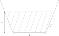
In Fig. 1, the variable $x$ denotes the spatial domain of the channel, while $Q(x,t)$ represents the water discharge, and $h(x,t)$ signifies the height of the water surface relative to the channel bottom. Both $Q(x,t)$ and $h(x,t)$ are dependent on both time and spatial domain. The head-on view of the channel’s cross-section is illustrated in Fig. 2, where $A(x,t)$ denotes the wet area, calculated from the channel bottom to the water surface. The wet perimeter is symbolized as $P$ , representing the circumference of the channel beneath the water surface. In accordance with Eq. (2), the variable $u$ corresponds to water velocity, which is contingent on both the spatial domain and time. Additionally, $S_f$ , as computed by the methodology outlined by Brunner (2021), corresponds to the friction slope of the channel and is calculated as follows:

Close

Fig. 1

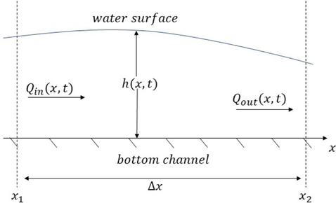
Side view of the water channel.

Export to PPT

Here, we modify Eqs. (1) and (2) by substituting $Q(x,t)=A(x,t)u(x,t)$ into the equations. Therefore, the following equations are obtained:

Close

Fig. 2

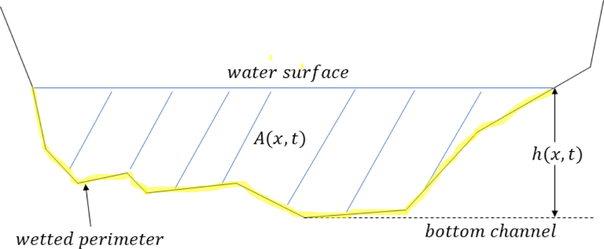
Front view of the water channel.

Export to PPT

Solving the Saint-Venant Equations explicitly is impractical, as it necessitates assumptions that do not accurately represent real-world scenarios, as noted in the work by Sleigh and Goodwill (2000). Consequently, the system of Eqs. (4) and (5) will be addressed through numerical methods. The chosen numerical approach for solving this system of equations is the Finite Volume on Staggered Grid Method.

3 Numerical scheme

The numerical schematic illustration is presented in Fig. 3. Supposing there is a channel of length $L$ , we define the spatial domain $[0,L]$ . Then, this spatial domain is partitioned into a grid where the partition points are $x_{\frac{1}{2}}=0,x_1,\dots ,x_{i-\frac{1}{2}},x_i,x_{i+\frac{1}{2}},\dots ,x_{N_x+\frac{1}{2}}=L$ . The number of partitions is written as $N_x=\lfloor \frac{L}{\Delta x}\rfloor +1$ , where $\Delta x$ represents the length of each partition. Eq. (4) will be calculated on points labeled $[x_{i-\frac{1}{2}},x_{i+\frac{1}{2}}]$ , marked in blue, and Eq. (5) will be calculated on points labeled $[x_i,x_{i+1}]$ , marked in red. Here, we calculate $A$ and $h$ on the full grid ( $x_i$ ), while $u$ and $S_f$ are calculated on the half grid ( $x_{i+\frac{1}{2}}$ ). This calculation is done in the spatial domain. Furthermore, the calculations are also done for a defined amount of time $T$ , so that we can define the time domain $[0,T]$ . The time domain is partitioned into $N_t=\lfloor \frac{T}{\Delta t}\rfloor +1$ points, where $\Delta t$ represents the numerical time step.

Close

Fig. 3

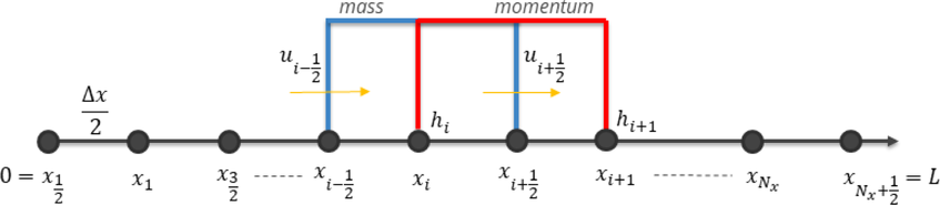
Illustration of the finite volume on staggered grid method.

Export to PPT

By using the Forward Time Centered Space (FTCS) method, Eqs. (4) and (5) can be approximated by

Notice that in Eq. (6), the value of $A$ in the half grid is needed to calculate ${\left(Au\right)}_{i+\frac{1}{2}}^n$ , but the value is missing because $A$ is calculated on the full grid. Therefore, we approach the required value of $A$ using the first-order upwind method, which depends on water flow velocity. The approximate value of $A$ is symbolized by ${}^{\ast }A$ as follows:

By substituting ${}^{\ast }{A}_{i+\frac{1}{2}}^n$ into Eq. (6) and simplifying the resulted equation, we obtain:

By substituting the value of ${\left(u{u}_x\right)}_{i+\frac{1}{2}}^n$ in Eq. (10) to Eq. (7) and simplifying the result for $u_{i+\frac{1}{2}}^{n+1}$ , we obtain:

The calculation of ${\left(S_f\right)}_{i+\frac{1}{2}}^n$ will take into account the shape of the channel’s cross-section. Eqs. (9) and (15) represent the discretized mass conservation and momentum balance equations, respectively, which will yield solutions for the variables $h$ and $u$ . Since the numerical computations are contingent on the shape of the channel’s cross-section, it is essential to examine the model developed for both regular and irregular channel sections.

3.1

3.1 Model for regular cross section

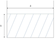
This research will scrutinize two distinct regular cross-sectional shapes: a rectangular channel and a trapezoidal channel. Table 1 delineates the method for computing the wet areas, wet perimeters, and hydraulic radius, for both rectangular and trapezoidal channel cross-section. Here, $b$ corresponds to the width of the channel’s bottom, $h$ signifies the height of the water surface, and $z$ characterizes the side slope in the case of a trapezoidal cross-section.

We can calculate the value of the water level by considering the wet area in Table 1. For the case with a rectangular cross-section, the water level follows

(16)

$$h_i^{n+1}=\frac{A_i^{n+1}}{b},$$ while for the case of a trapezoidal cross-section, it follows

(17)

$$h_i^{n+1}=\frac{A_i^{n+1}}{b+z{h}_i^n}.$$ Next, the value of ${\left(S_f\right)}_{i+\frac{1}{2}}^n$ is calculated by considering the hydraulic radius in Table 1 and Eq. (3). The discrete form of Eq. (3) is

(18)

$${\left(S_f\right)}_{i+\frac{1}{2}}^n=\frac{u_{i+\frac{1}{2}}^n\left|u_{i+\frac{1}{2}}^n\right|n_f^2}{{\left(R_{i+\frac{1}{2}}^n\right)}^{4/3}}.$$ For the rectangular cross-section, the following applies:

(19)

$$R_{i+\frac{1}{2}}^n=\frac{b{{}^{\ast }h}_{i+\frac{1}{2}}^n}{b+2{{}^{\ast }h}_{i+\frac{1}{2}}^n},$$ whereas for the trapezoidal cross-section,

(20)

$$R_{i+\frac{1}{2}}^n=\frac{(b+z{{}^{\ast }h}_{i+\frac{1}{2}}^n){{}^{\ast }h}_{i+\frac{1}{2}}^n}{(b+2{{}^{\ast }h}_{i+\frac{1}{2}}^n)\sqrt{1+z^2}},$$ where

(21)

$${{}^{\ast }h}_{i+\frac{1}{2}}^n=\left\{\begin{array}{c}{h}_i^n,u_{i+\frac{1}{2}}^n\ge 0,\hfill \\ h_{i+1}^n,u_{i+\frac{1}{2}}^n<0.\hfill \end{array}\right.$$

Table 1 The formulas to determine wet areas, wet perimeters, and hydraulic radius of rectangular and trapezoidal cross-sections.

Cross section	Wet area ( $A$ )	Wet perimeter ( $P$ )	Hydraulic radius ( $R$ )
	$bh$	$b+2h$	$\frac{bh}{b+2h}$
	$(b+zh)h$	$(b+2h)\sqrt{1+z^2}$	$\frac{(b+zh)h}{(b+2h)\sqrt{1+z^2}}$

3.2

3.2 Model for irregular cross section

In the case of an irregular channel cross-section, it is not feasible to obtain the exact formulas for directly calculating $h$ , $A$ , and $R$ , as is done in the regular section approach. Instead, the Riemann Sum Partitioning Method is employed. An illustration of this method is provided Fig. 4.

Suppose the objective is to solve the wet area of Fig. 4. The approximation of this area is the sum of the areas of all rectangular bands, which are symbolized by $A_1,A_2,A_3,\dots ,A_j,\dots ,A_{N_p}$ . The number of partitions is $N_p=\frac{B}{\Delta b}$ , where $\Delta b$ is the partition width (bandwidth). Suppose $y_j$ is the distance from the $j^{th}$ partitioned channel cross-section to the bottom of the channel. Then,

(22)

$$h=\frac{\frac{A}{\Delta b}+y_1+y_2+y_3+\cdots +y_{N_p}}{N_p}.$$ The equation for calculating $h$ for an irregular cross-sectional channel is

(23)

$$h_i^{n+1}=\frac{1}{N_p}\left(\frac{A_i^{n+1}}{\Delta b}+\sum _{j=1}^{N_p}{y}_j\right).$$

Close

Fig. 4

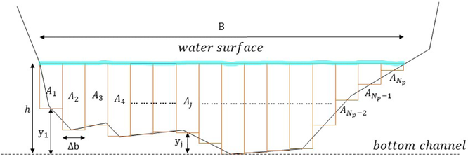
Illustration of the Riemann Sum Partitioning Method.

Export to PPT

Next, to calculate the value of $S_f$ , we need the value of the hydraulic radius ( $R$ ). Since the channel’s cross section is irregular, we can use the formula $\left(wetarea\right)/\left(wetperimeter\right)$ to calculate the hydraulic radius. The wet area ( $A$ ) can be found using the equation that is also obtained from the above explanation, read as

(24)

$$A_{i+\frac{1}{2}}^n=\Delta b\left(\sum _{j=1}^{N_p}(\ast h_{i+\frac{1}{2}}^n-y_j)\right).$$ The wet perimeter ( $P$ ) can be calculated using the following equation:

(25)

$$P_{i+\frac{1}{2}}^n=2{{}^{\ast }h}_{i+\frac{1}{2}}^n-y_1-y_{N_p}+P_1+P_2+P_3+P_4,$$ where

(26)

$$P_1=\left(\sum _{j=1,y_j\ge y_{j-1}and{y}_j\ge y_{j+1}}^{N_p}\left(\Delta b\right)\right),$$

(27)

$$P_2=\left(\sum _{j=1,y_j<y_{j-1}and{y}_j\ge y_{j+1}}^{N_p}(\Delta b-y_j+y_{j-1})\right),$$

(28)

$$P_3=\left(\sum _{j=1,y_j\ge y_{j-1}and{y}_j<y_{j+1}}^{N_p}(\Delta b-y_j+y_{j+1})\right),$$

(29)

$$P_4=\left(\sum _{j=1,y_j<y_{j-1}and{y}_j<y_{j+1}}^{N_p}(\Delta b-2y_j+y_{j-1}+y_{j+1})\right).$$ Therefore, the equation for discretized hydraulic radius is

(30)

$$R_{i+\frac{1}{2}}^n=\frac{A_{i+\frac{1}{2}}^n}{P_{i+\frac{1}{2}}^n}.$$

The formulated numerical scheme is then converted into a program code developed in MATLAB to conduct several simulations. To validate the scheme’s accuracy and performance, the results of these simulations are then compared with both laboratory experiments and the HEC-RAS application.

4 Experiment and result

4.1

4.1 Comparisons against experimental data

The experiments were conducted at the Water Resources Engineering Laboratory, Bandung Institute of Technology, Bandung, Indonesia, using a rectangular flume of $7.5\mathrm{cm}$ wide, $600\mathrm{cm}$ long, and $24\mathrm{cm}$ high, as depicted in Fig. 5. In addition, a pitot tube was employed to measure the upstream water discharge. The water flow simulations were captured using a camera, and the numerical data generated by HEC-RAS was extracted through the utilization of CurveSnap software. The observation area covered the range of 0–132 $\mathrm{cm}$ measured from the upstream. Two scenarios were included in the experiments: the first involved creating a blockage at the flume’s downstream end, which generated a reflected wave, and the second scenario entailed the free flow downstream.

Close

Fig. 5

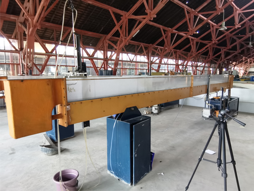
The rectangular wave flume used in the experiments.

Export to PPT

4.1.1

4.1.1 The first simulation case

During the initial simulation, the wave pump was operated for $15$ seconds to initiate water flow. Subsequently, the pump was deactivated for $7$ seconds. Using the pitot tube, the water discharge at the upstream-end was recorded at $13.288{\mathrm{cm}}^3/\mathrm{s}$ over the first $15$ seconds. The initial water surface level was set at $6\mathrm{cm}$ . The blockage was positioned at a distance of $587,5\mathrm{cm}$ from the upstream-end. Consequently, the parameters for the numerical scheme are as follows:

• $\Delta x=20\mathrm{cm}$

• $\Delta t=0.01\mathrm{s}$

• $\Delta b=0.075\mathrm{cm}$

• $g=981\mathrm{cm}/{\mathrm{s}}^2$

• $n_f=0.005$

• Upstream boundary condition:

  (31)
  $$u_0^t=\left\{\begin{array}{c}13.288,t\le 15,\hfill \\ 1.5,15<t\le 22.\hfill \end{array}\right.$$

• Downstream boundary condition:

  (32)
  $$u_{N_x+\frac{1}{2}}^t=0,t>0.$$

4.1.2

4.1.2 The second simulation case

For the second simulation, the wave pump was operated continuously for $60$ seconds without any interruption. Consequently, the upstream water discharge remained at a constant rate of $13.288{\mathrm{cm}}^3/\mathrm{s}$ throughout the entire duration. The initial water surface level, $\Delta x$ , $\Delta t$ , $\Delta b$ , $g$ , and $n_f$ , were maintained the same as in the first simulation. Additionally, the following parameters are applicable for this second scenario:

• Upstream boundary condition:

  (33)
  $$u_0^t=13.288,t>0.$$

• The downstream boundary condition for free flow is constructed by extending the spatial domain with a large value.

After we got the experimental data, we conducted numerical simulations in MATLAB with the same parameters as the experiment and compared both results. Fig. 6 illustrates that both the irregular and regular models yield highly satisfactory results, a finding that aligns well with the experimental data. The water levels generated by both the irregular and regular models exhibit a consistent and similar trend when compared to the water levels observed during the experiments. Moreover, the water level values in the irregular model consistently match those of the regular model. Consequently, it can be deduced that the irregular model has been effectively calibrated and can be deemed reliable for addressing analogous scenarios. In addition, based on the results of the experiments, it was observed that the model’s parameters cannot be excessively small. To address this issue, we converted all parameter units to the C.G.S. unit system in order to yield larger values. Additionally, our findings indicate a tendency for the time step ( $\Delta t$ ) to be smaller than the spatial step ( $\Delta x$ ).

Close

Fig. 6

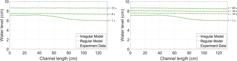
Comparisons between the simulation results and experimental data for the first (left) and second (right) case.

Export to PPT

4.2

4.2 Comparisons against the results from HEC-RAS

In addition to the previous validation efforts, comparisons between the results of our model and those of HEC-RAS software have been carried out. The overarching simulation scheme encompasses water flowing from upstream to downstream with a specific discharge rate, covering a channel with a length of $10000$ m over a duration of $2$ h. The Manning coefficient assigned to the channel is 0.02. This section will focus on the evaluation of three different channel’s cross-sections: a trapezoidal channel, and two distinct irregular channels, as depicted in Fig. 7.

Close

Fig. 7

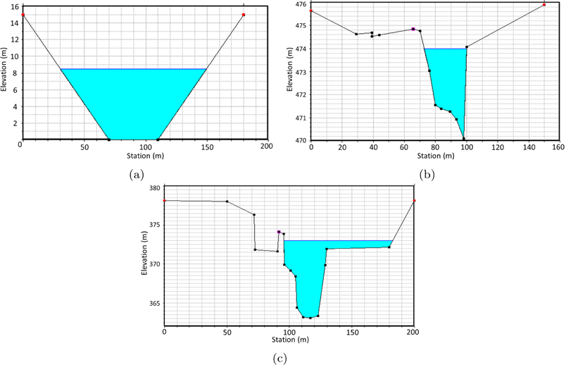
Front view of the assessed channels.

Export to PPT

4.2.1

4.2.1 Trapezoidal channel

The configuration and dimensions of this cross-section are depicted in Fig. 7(a). The initial water level is set at 8.5 m. The upstream boundary condition is gradually increased from 300 ${\mathrm{m}}^3/\mathrm{s}$ to 500 ${\mathrm{m}}^3/\mathrm{s}$ , and the downstream boundary condition is held constant at 200 ${\mathrm{m}}^3/\mathrm{s}$ . The results and the comparative analysis between the irregular model, regular model, and HEC-RAS are presented in Fig. 8(a).

4.2.2

4.2.2 First irregular channel

The shape and dimensions of the first irregular cross-section are visualized in Fig. 7(b). The initial water level stands at $474$ meters. The upstream boundary condition is incrementally raised from $20{\mathrm{m}}^3/\mathrm{s}$ to $40{\mathrm{m}}^3/\mathrm{s}$ during the first hour, and then gradually decreased to $30{\mathrm{m}}^3/\mathrm{s}$ in the second hour. The downstream boundary condition remains constant at $0{\mathrm{m}}^3/\mathrm{s}$ . As there is no exact formula for calculating the area of an irregular shape, the irregular model is exclusively used in this case. The results and the comparative analysis between the irregular model and HEC-RAS can be found in Fig. 8(b).

4.2.3

4.2.3 Second irregular channel

The configuration and dimensions of the second irregular cross-section are shown in Fig. 7(c). The initial water level is set at $373$ meters. The upstream boundary condition is progressively increased from $185{\mathrm{m}}^3/\mathrm{s}$ to $441{\mathrm{m}}^3/\mathrm{s}$ in the first hour, and then gradually decreased to $263{\mathrm{m}}^3/\mathrm{s}$ in the second hour. The downstream boundary condition is maintained at a constant rate of $189{\mathrm{m}}^3/\mathrm{s}$ . In this case, only the irregular model is employed, given the absence of an exact formula for determining the area of an irregular shape. The results and the comparative analysis between the irregular model and HEC-RAS are displayed in Fig. 8(c).

Fig. 8(a) demonstrates that both the regular and irregular models align closely with the results obtained from HEC-RAS in the case of the trapezoidal cross-section, although minor differences in water levels are apparent during the first hour. Furthermore, it is noteworthy that the irregular model consistently produces results matching those of the regular model, affirming the adequacy of the irregular model’s approximation for the trapezoidal cross-section.

Close

Fig. 8

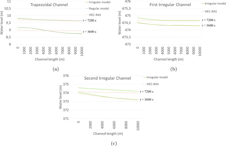
Comparisons between the results generated by the developed model and HEC-RAS in various types of channels.

Export to PPT

Figs. 8(b) and 8(c) reveal that for the complex cross-sectional channels, the irregular model provides satisfactory results when compared to HEC-RAS, with only slight disparities in water levels between the irregular model and HEC-RAS. These observations collectively indicate that the irregular model is a dependable and credible tool for modeling water flow in irregular channels.

Close

Fig. 9

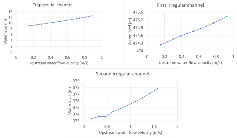
The relationship of upstream water flow velocity with the average water level at the end of the simulation in various type of channels.

Export to PPT

From these comparisons, we notice that the values of parameters $\Delta x$ , $\Delta t$ , and $\Delta b$ , have important roles in the results of our model. These parameters affect the computation time and stability condition. We use a trial-and-error method to define the value of $\Delta x$ and $\Delta t$ based on the Courant–Friedrichs–Lewy condition for Eqs. (4) and (5), which is $\sqrt{g{h}_{max}}\frac{\Delta t}{\Delta x}$ (Magdalena et al., 2021b). For $\Delta b$ , we can use the smallest possible value as long as it does not take a long calculation time. Once the model has an optimal value for $\Delta x$ , $\Delta t$ , and $\Delta b$ , we can get a good enough result, as explained above. Unfortunately, this model has a limitation; not all cases can be simulated by it. For example, when the initial water level value is very small but the incoming water discharge is very large, the model becomes unstable. For this case, we suggest doing a further comparison to another model like HEC-RAS.

5 Conclusions

The numerical model we proposed based on the Saint-Venant Equations excels at replicating real-world conditions, showcasing its efficacy in comparison to experimental data. Furthermore, when evaluated against HEC-RAS software, our model consistently yields highly compatible outcomes, characterized by minimal discrepancies in water level. The unique advantage of the irregular model lies in its adaptability to a diverse array of cross-sectional geometries. When equipped with coordinate data for cross-sectional geometry, it readily accommodates the modeling of rivers or channels of virtually any shape. Additionally, our model is well-suited to investigate scenarios in which fluctuations in water discharge substantially affect watershed flooding, a dynamic that can be observed by manipulating water discharge values over the course of the simulations. Lastly, sensitivity analysis elucidates that a closed downstream area invariably results in a linear relationship between upstream water flow velocity and water level at the end of the simulation.

Our findings demonstrate that the water level in an open channel is influenced by several key factors, including water discharge, channel’s slope, friction, the initial water level, and the cross-sectional geometry of the channel. However, it is noteworthy that the primary factor affecting water level is water velocity, which is derived from the relationship between water discharge and wet area ( $Q=Au$ ). This is evident in the results of the first irregular channel case, where the given water discharge is smaller compared to other cases, but the rise in water level is closely parallel to that of other cases with smaller cross-sectional areas. Hence, when the wet area is reduced, the increase in water level occurs more rapidly.

CRediT authorship contribution statement

I. Magdalena: Conceptualization, Data curation, Formal analysis, Funding acquisition, Methodology, Project administration, Resources, Software, Supervision, Writing – review & editing. Riswansyah Imawan: Data curation, Formal analysis, Investigation, Methodology, Validation, Visualization, Writing – original draft. M. Adecar Nugroho: Data curation, Formal analysis, Project administration, Resources, Supervision, Writing – review & editing.

References

- Mathematical and numerical modelling of shallow water flow. Comput. Mech.. 1993;11:280-299.
- [Google Scholar]
- A functional autoregressive model based on exogenous hydrometeorological variables for river flow prediction. J. Hydrol.. 2021;598:126380
- HEC-RAS, River Analysis System Hydraulic Reference Manual. US Army Corps of Engineers Hydrologic Engineering Center (HEC); 2021.
- Numerical simulation of two-layer shallow water flows through channels with irregular geometry. J. Comput. Phys.. 2004;195:202-235.
- A new approach to model weakly nonhydrostatic shallow water flows in open channels with smoothed particle hydrodynamics. J. Hydrol.. 2014;519:1010-1019.
- Numerical simulation of shallow-water dam break flows in open channels using smoothed particle hydrodynamics. J. Hydrol.. 2011;408:78-90.
- Balanced finite volume WENO and central WENO schemes for the shallow water and the open-channel flow equations. J. Comput. Phys.. 2004;200:512-548.
- Between hydrodynamics and elasticity theory: The first five births of the Navier-Stokes equation. Arch. Hist. Exact Sci.. 2002;56(2):95-150.
- Case study of HEC-RAS 1D–2D coupling simulation: 2002 baeksan flood event in Korea. Water. 2019;11:2048.
- Sediment transport models in shallow water equations and numerical approach by high order finite volume methods. Comput. & Fluids. 2008;37:299-316.
- Flood modeling of a large transboundary river using WRF-Hydro and microwave remote sensing. J. Hydrol.. 2021;598:126391
- Some recent developments in turbulence closure modeling. Annu. Rev. Fluid Mech.. 2018;50:77-103.
- An extended Boussinesq theory for interfacial fluid mechanics. J. Engrg. Math.. 2022;133:10.
- Comparison of 1D and 2D hydraulic models for floods simulation on the Medjerda Riverin Tunisia. J. Mater. Environ. Sci.. 2016;7(8):3017-3026.
- An extended form of Boussinesq-type equations for nonlinear water waves. J. Hydrodynam. Ser. B. 2015;27(5):696-707.
- Modeling of unsteady flow through junction in rectangular channels: Impact of model junction in the downstream channel hydrograph. Sci. Res. Publ.. 2017;6:304-319.
- Grid-based simulation of river flows in Northern Ireland: Model performance and future flow changes. J. Hydrol.: Reg. Stud.. 2021;38:100967
- Irregular wave propagation with a 2DH Boussinesq-type model and an unstructured finite volume scheme. Eur. J. Mech. B Fluids. 2018;72:432-448.
- Channel responses to flooding of Ganga River, Bihar India, 2019 using SAR and optical remote sensing. Adv. Space Res.. 2022;69:1930-1947.
- Modeling and Control of Hydrosystems. Springer; 2009.
- A new form of the Boussinesq equations with improved linear dispersion characteristics. Part 2. A slowly-varying bathymetry. Coast. Eng.. 1992;18(3–4):183-204.
- Numerical approaches for Boussinesq type equations with its application in Kampar River, Indonesia. Math. Comput. Simulation 2023
- Numerical studies of dam break flow with an obstacle through different geometries. Results Appl. Math.. 2021;12:100193
- Water waves resonance and its interaction with submerged breakwater. Results Eng.. 2022;13:100343
- A mathematical model for investigating the resonance phenomenon in lakes. Wave Motion 2021
- Quantification of wave attenuation in mangroves in Manila Bay using nonlinear Shallow Water equations. Results Appl. Math.. 2021;12:100191
- Two layer shallow water equations for wave attenuation of a submerged porous breakwater. Appl. Math. Comput.. 2023;454:128096
- Analytical and numerical studies for Seiches in a closed basin with bottom friction. Theor. Appl. Mech. Lett.. 2020;10(6):429-437.
- Review of the shear-stress transport turbulence model experience from an industrial perspective. Int. J. Comput. Fluid Dynam.. 2009;23(4):305-316.
- Saint-venant model analysis of trapezoidal open channel water flow using finite difference method. Procedia Comput. Sci.. 2019;157:6-15.
- Alternative form of Boussinesq equations for nearshore wave propagation. J. Waterw. Port Coast. Ocean Eng.. 1993;119(6)
- Absorbing boundary condition for nonlinear hyperbolic partial differential equations with unknown Riemann invariants. Mecanica Comput.. 2009;28:1593-1620.
- Hydraulic and hydrologic analysis of unsteady flow in prismatic open channel. Proc. MDPI. 2018;2(11):571.
- The st venant equations. 2000. Leeds School of Civil Engineering University of Leeds England
- High order well-balanced finite difference WENO schemes for shallow water flows along channels with irregular geometry. Appl. Math. Comput.. 2019;363:124587
- Partition of one-dimensional river flood routing uncertainty due to boundary conditions and riverbed roughness. J. Hydrol.. 2022;608:127660
- High order finite volume WENO schemes for the shallow water flows through channels with irregular geometry. J. Comput. Appl. Math.. 2016;299:229-244.
- Modelling open-channel flow with rigid vegetation based on two-dimensional shallow water equations using the lattice Boltzmann method. Ecol. Eng.. 2017;106:75-81.
- Modified Saint-Venant equations for flow simulation in tidal rivers. Water Sci. Eng.. 2012;5(1):34-45.