1 Introduction

Use of orthogonal polynomials in the Rayleigh–Ritz method for solving most of the important differential equations has attracted the researcher's interest since 19th century. Many studies on the vibration of non-rectangular plates assuming various deflection shape functions in the Rayleigh–Ritz method have been reported by Leissa (1969). Following the publications of Szego's well known treatise Szego (1967) and Singh and Chakraverty (1991, 1992, 1993, 1994a,b) there has been tremendous growth of literature covering various aspects of the subject but, unfortunately, for plates of uniform boundary conditions. Sato (1973) presented experimental as well as theoretical results for elliptic plates but again with uniform free edge. An interesting contribution in this regard has been done by Bhat et al. (1998) and Chakraverty et al. (1999). They presented a recurrence scheme that makes the generation of two-dimensional boundary characteristic orthogonal polynomials for a variety of geometries straight forward and quite efficient. They also provide a survey of the application of BCOPs method in vibration problems. Some important books on orthogonal polynomials and its applications are Beckmann (1973), Chihara (1978), and Gautschi et al. (1999).

There is no analytical solution to the vibration problems of plates with non-uniform boundary conditions even for plates of simple geometrical shapes like rectangles (Wei et al., 2001). Very little is available in literature on elliptical plates with non-uniform boundary conditions and, whenever available, it is mostly on circular plates. That is why this kind of problems has become a challenging problem for scientists and engineers. Some available references are Eastep and Hemmig (1982), Hemmig (1975), Leissa et al. (1979), Laura and Ficcadenti (1981) and Narita and Leissa (1981). Hassan (2007) has generated BCOPs to compute natural frequencies of an elliptical plate with half of the boundary simply supported and the rest free and gave numerical and graphical results for this case. In Hassan (2004) he solved the vibration problem under consideration by using traditional basis functions that satisfy the essential boundary conditions of the CF-elliptical plate in the Rayleigh–Ritz method. Explicit numerical and graphical results have been given and reported for the first time. Other publications dealing with plates with mixed boundary conditions have been recently appeared by Boborykin (2006), Czernous (2006), and Zovatto and Nicolini (2006). They investigated the bending problem of a rectangular plate with mixed boundary conditions. No numerical results are available for vibrations of elliptical plates with mixed boundary conditions.

The aim of the present work is to generate a sequence of boundary characteristic orthogonal polynomials over an elliptical domain occupied by a thin elastic plate with half of the boundary, $y⩽0$ , clamped and the rest free. These polynomials should satisfy at least the essential boundary conditions of the problem. The coefficients of these polynomials will be generated and tabulated in advance, once and for all, with the desired precision. Use of these polynomials in Rayliegh–Ritz method helped in presenting explicit numerical results for the problem under consideration. This method reduces ill-conditioning of the resulting system whose solution has become comparatively easier and faster in convergence. Three-dimensional solution surfaces, mode shapes, and the associated contour lines of the problem have been plotted in some selected cases. Comparison of results have been made with known results in literature whenever available.

2 Generation of boundary characteristic orthogonal polynomials

As has been done by Bhat (1985) for one-dimensional orthogonal polynomials and by Liew et al. (1990) for rectangular plates one will follow the same procedures to generate a set of orthogonal polynomials in two variables over an elliptical domain $R^{\prime }$ occupied by a thin elastic plate in the xy-plane with half of the boundary, $y⩽0$ , clamped and the rest free. For this one can start with the set of linearly independent functions

3 Rayleigh–Ritz procedures

For a plate undergoing simple harmonic motion equating the maximum strain energy $V_{\mathit{max}}$ and the maximum kinetic energy $T_{\mathit{max}}$ of the deformed plate the Rayleigh quotient (see Siddiqi, 2004) is

4 Numerical results and discussion

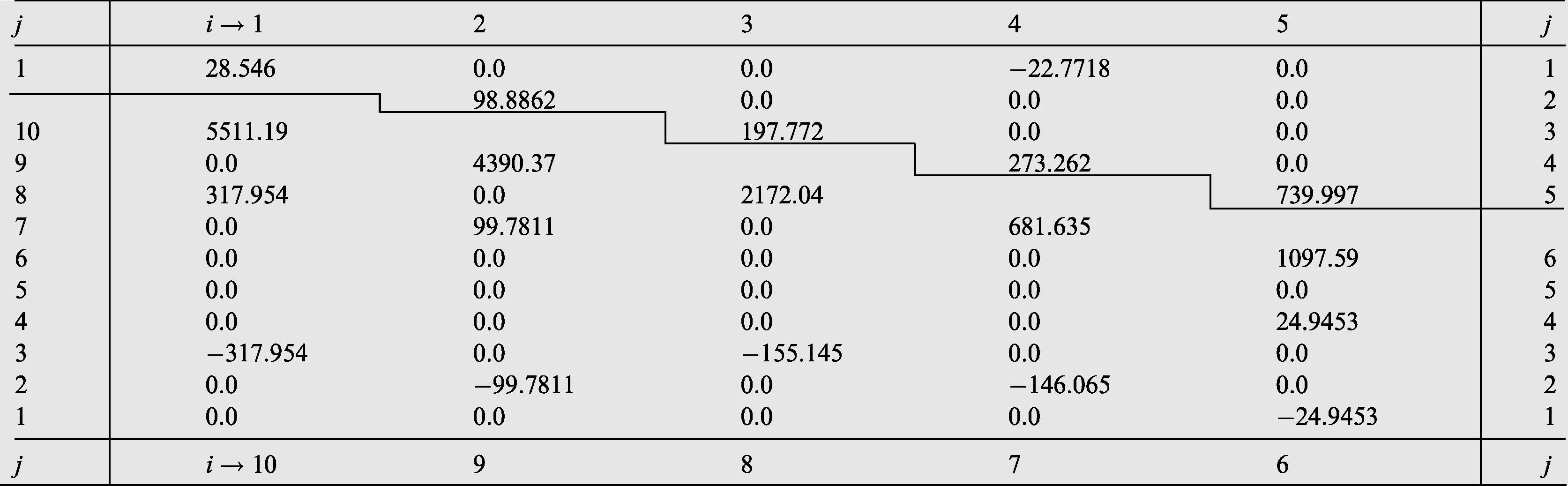
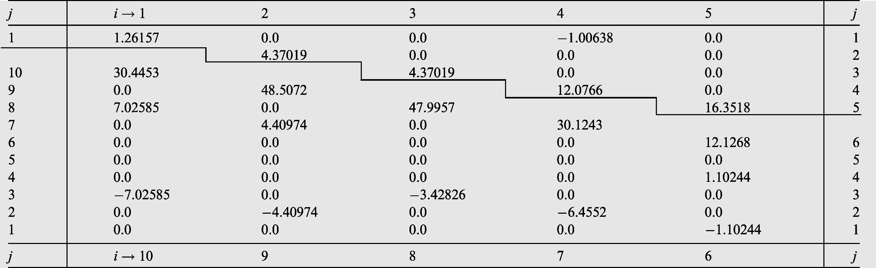
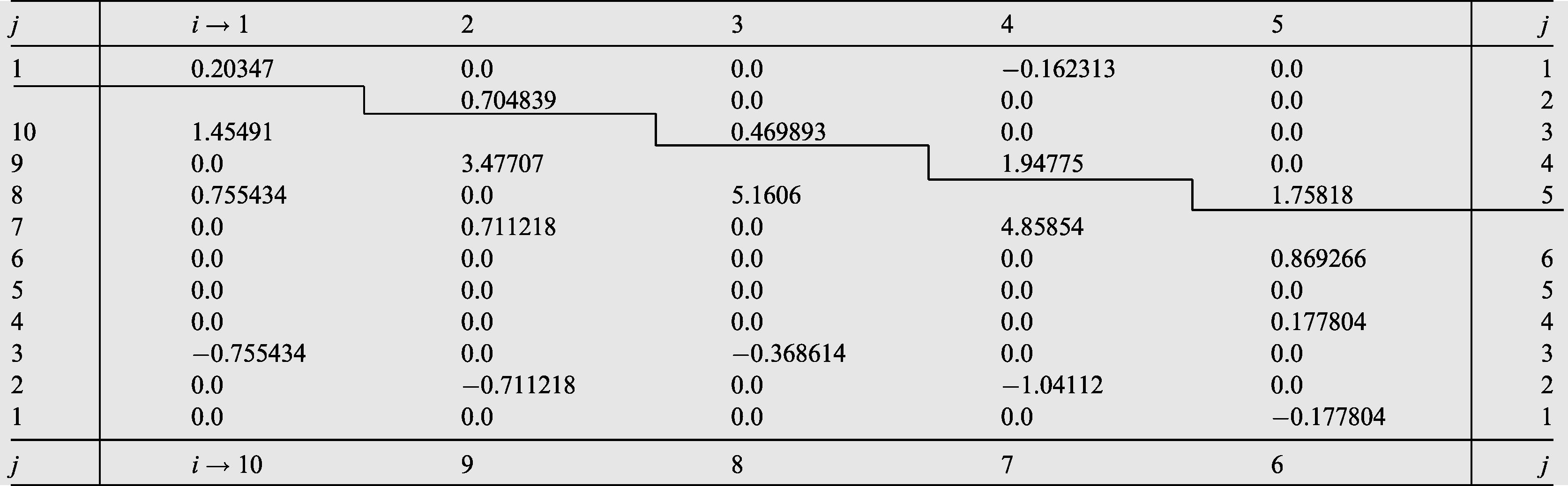
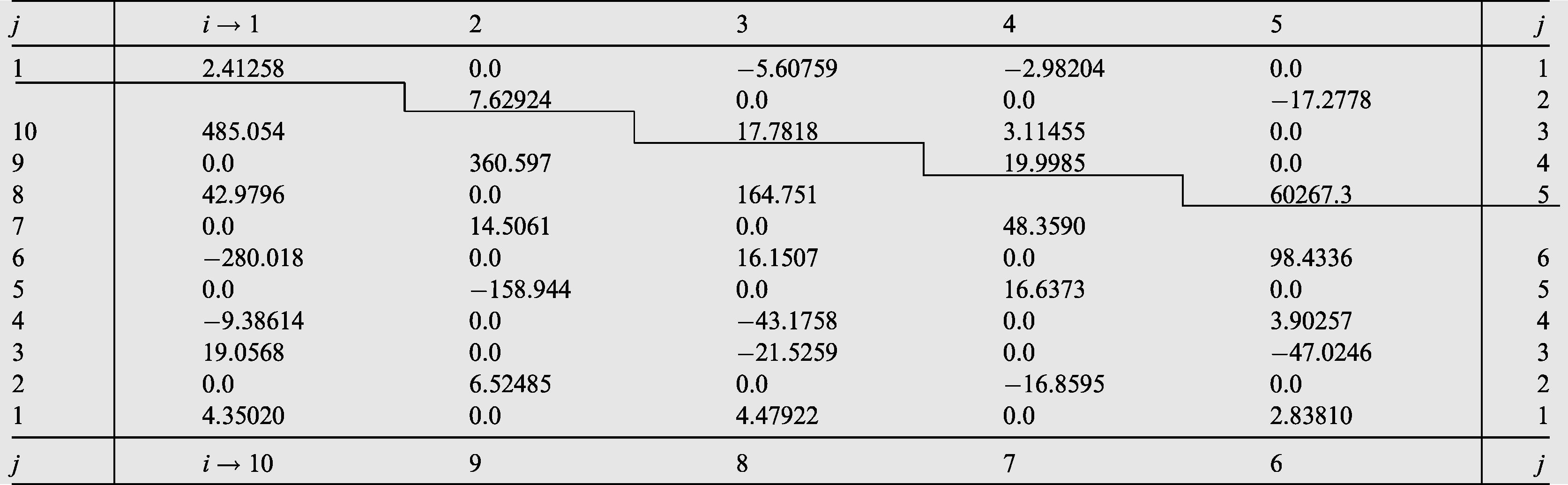
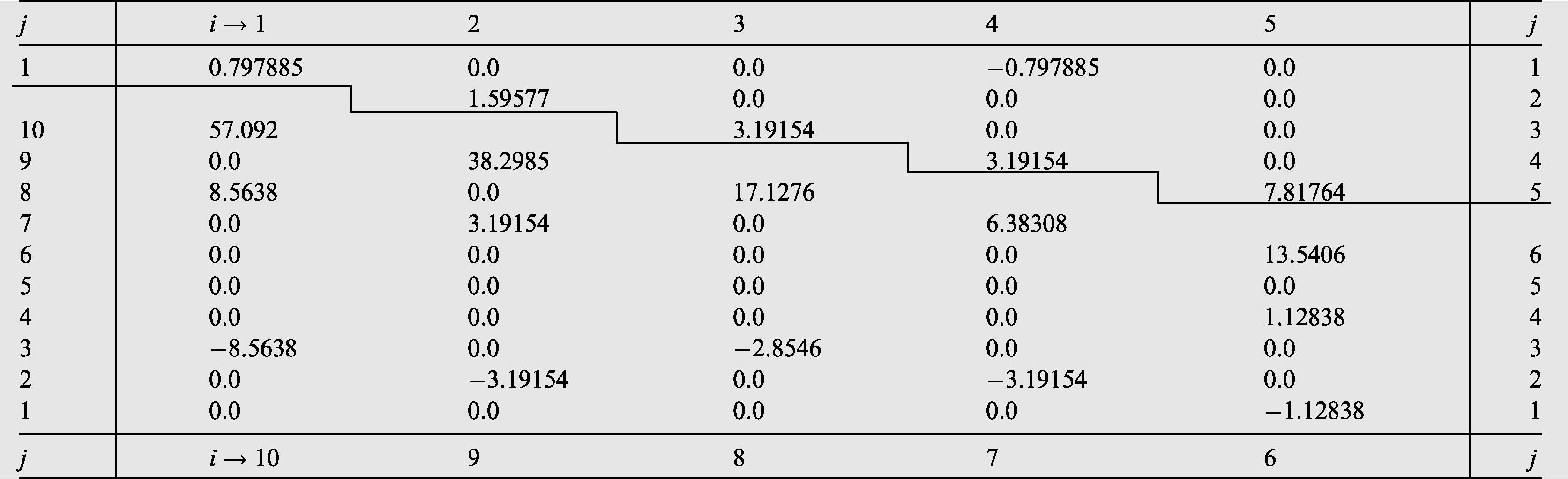
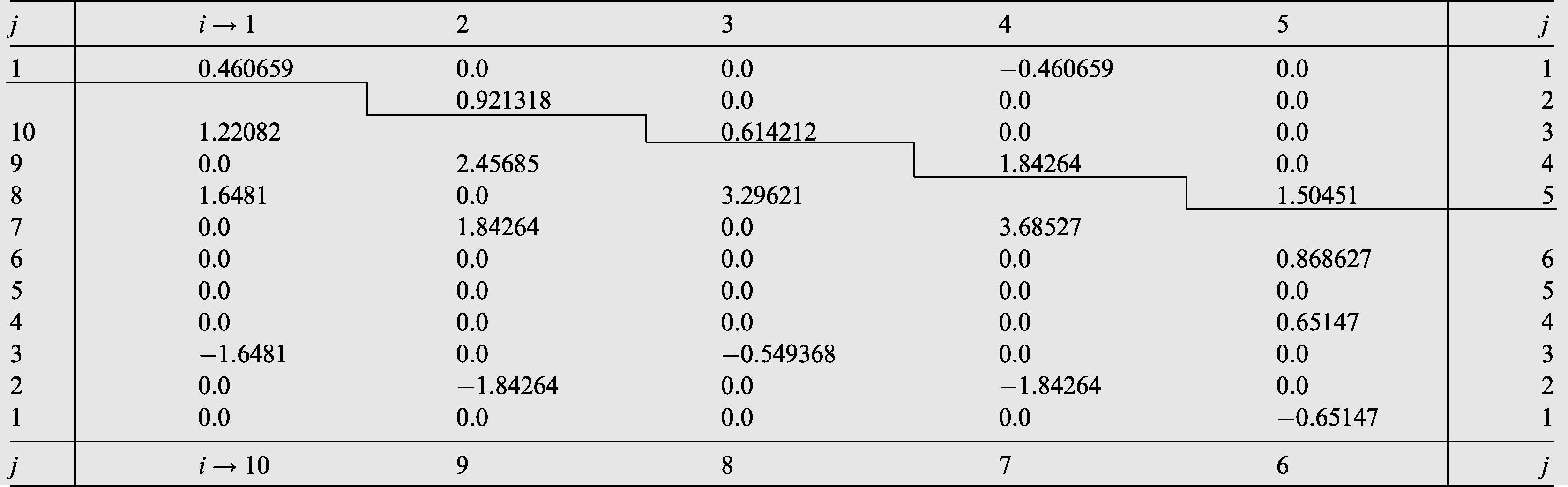
The function u in (2) has been so chosen that the essential boundary conditions of the elliptical plate are satisfied. Consequently the essential boundary conditions of the problem are thus satisfied by the functions $F_i(X\text{,}Y)$ also. Finally BCOPs can be expressed in terms of $f_i$ by computing ${\beta }_{\mathit{ij}}$ in (8). All the computations have been worked out by using Mathematica 5.2 on a PC. This greatly simplifies and reduces the huge effort spent in preparing lengthy computations and cumbersome programs in any programming high level language. Also one can examine directly and easily the validity of the chosen function u whether it is suitable to our case or not without repeating the hall calculations from the very beginning in case one face any integration problems. Moreover, it enables one to use variation functions other than polynomial variations without fear of the integrals involved (for further work). The coefficients ${\hat{\beta }}_{\mathit{ij}}$ of the orthonormal polynomials have been computed and reported in Tables 1–4 which correspond to the aspect ratios $r=0.5\text{,}1.0\text{,}1.5$ and 2.0, respectively, for CC-elliptical plate. Tables 5–8 are for CF-elliptical plate and Tables 9–12 are for FF-elliptical plate. The case $r=1.0$ corresponds to a circular plate. It is to be noted that the program can generate results for any value of the aspect ratio $r>0$ . The approximation order N has been increased from 1 to 28 for CC and FF-cases but from 1 to 10 only in the CF-case. It is a gigantic task to go through approximations beyond this because of the singularities arising in some integrals due to discontinuities at $X=\pm 1$ . If it is necessary the recurrence scheme mentioned in Bhat et al. (1998) is recommended, for further work, which makes the generation of orthogonal polynomials easier and straight forward. For need of space only 10 polynomials have been reported in all cases. The tabulated coefficients have been computed once for all and the reader can use these directly without repeating the calculations again and again. As a check on accuracy of the results it has been verified that

Table 1 Coefficients ${\hat{\beta }}_{\mathit{ij}}$ of first 10-polynomials ${\hat{\varphi }}_i$ for CC-elliptical plate with $r=0.5$ , and $\nu =0.3$ .

Table 2 Coefficients ${\hat{\beta }}_{\mathit{ij}}$ of first 10-polynomials ${\hat{\varphi }}_i$ for CC-elliptical plate with $r=1$ , and $\nu =0.3$ .

Table 3 Coefficients ${\hat{\beta }}_{\mathit{ij}}$ of first 10-polynomials ${\hat{\varphi }}_i$ for CC-elliptical plate with $r=1.5$ , and $\nu =0.3$ .

Table 4 Coefficients ${\hat{\beta }}_{\mathit{ij}}$ of first 10-polynomials ${\hat{\varphi }}_i$ for CC-elliptical plate with $r=2$ , and $\nu =0.3$ .

Table 5 Coefficients ${\hat{\beta }}_{\mathit{ij}}$ of first 10-polynomials ${\hat{\varphi }}_i$ for CF-elliptical plate with $r=0.5$ , and $\nu =0.3$ .

Table 6 Coefficients ${\hat{\beta }}_{\mathit{ij}}$ of first 10-polynomials ${\hat{\varphi }}_i$ for CF-elliptical plate with $r=1.0$ , and $\nu =0.3$ .

Table 7 Coefficients ${\hat{\beta }}_{\mathit{ij}}$ of first 10-polynomials ${\hat{\varphi }}_i$ for CF-elliptical plate with $r=1.5$ , and $\nu =0.3$ .

Table 8 Coefficients ${\hat{\beta }}_{\mathit{ij}}$ of first 10-polynomials ${\hat{\varphi }}_i$ for CF-elliptical plate with $r=2.0$ , and $\nu =0.3$ .

Table 9 Coefficients ${\hat{\beta }}_{\mathit{ij}}$ of first 10-polynomials ${\hat{\varphi }}_i$ for FF-elliptical plate with $r=0.5$ , and $\nu =0.3$ .

Table 10 Coefficients ${\hat{\beta }}_{\mathit{ij}}$ of first 10-polynomials ${\hat{\varphi }}_i$ for FF-plate with $r=1$ , and $\nu =0.3$ .

Table 11 Coefficients ${\hat{\beta }}_{\mathit{ij}}$ of first 10-polynomials ${\hat{\varphi }}_i$ for FF-elliptical plate with $r=1.5$ , and $\nu =0.3$ .

Table 12 Coefficients ${\hat{\beta }}_{\mathit{ij}}$ of first 10-polynomials ${\hat{\varphi }}_i$ for FF-elliptical plate with $r=2$ , and $\nu =0.3$ .

5 Mode shapes

Fig. 1a–f depict the first six mode shapes and the associated contour lines for a CF-elliptical plate with $r=0.5$ and $\nu =0.33$ . Figures corresponding to $\nu =0.3$ are roughly the same. These have been plotted by using tools of Computer Graphics under Turbo C++. The author has prepared his own software for that purpose. Other more figures corresponding to different aspect ratios are available in Hassan (2004).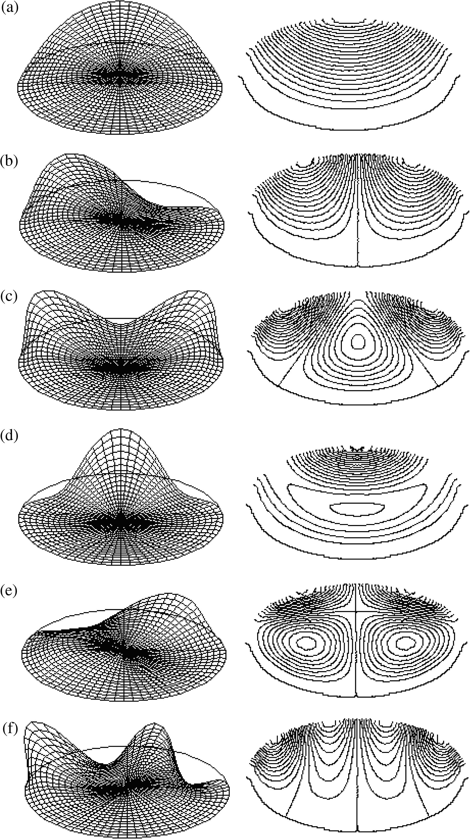

Close

Figure 1

First six mode shapes and the associated contour lines for CF-elliptical plate with $r=0.5$ and $\nu =0.33$ .

Export to PPT

6 Conclusion

The author has presented a set of orthonormal bases functions that can help in solving numerically the vibration problem of an elliptical plate clamped on lower half of the boundary and free on the upper half. Interested readers can use these directly without repeating the calculations again and again for similar problems. Those polynomials are not only simplifying the calculations but also minimizes the effects of ill-conditioning which frequently occurs with such problems since the resulting eigenvalue problem is no longer the generalized one now.

References

- Orthogonal Polynomials for Engineers and Physists. Golem Press; 1973.
- Natural frequencies of rectangular plates using characteristic orthogonal polynomials in Rayleigh–Ritz method. J. Sound Vib.. 1985;102:493-499.
- [Google Scholar]
- Recurrence scheme for the generation of two-dimensional boundary characteristic orthogonal polynomials to study vibration of plates. J. Sound Vib.. 1998;216(2):321-327.
- Solving the elastic bending problem for a plate with mixed boundary conditions. Int. J. Appl. Mech.. 2006;42(5):582-588.
- Recent research on vibration of structures using boundary characteristic orthogonal polynomials in the Rayleigh–Ritz method. Shock Vib. Dig.. 1999;13(3):187-194.
- An Introduction to Orthogonal Polynomials. London: Gordon and Breach; 1978.
- Generalized solutions of mixed problems for first-order partial functional differential equations. Ukrainian Math. J.. 2006;58(6):904-936.
- Natural frequencies of circular plates with partially free, partially clamped edges. J. Sound Vib.. 1982;84(3):359-370.
- Applications and computation of orthogonal polynomials. In: Conference at the Mathematical Research Institute Oberwolfach, Germany 22–28. Basel, Switzerland: Birkhauser; 1999.
- Free transverse vibration of elliptical plates of variable thickness with half of the boundary clamped and the rest free. Int. J. Mech. Sci.. 2004;46:1861-1882.
- Generating BCOPs to compute natural frequencies of an elliptical plate with half of the boundary simply supported and the rest free. Appl. Math. Inform. Sci. – An Int. J.. 2007;1(2):113-127.
- Hemmig, F.G., 1975. Investigation of natural frequencies of circular plates with mixed boundary conditions. Air Force Institute of Technology, School of Engineering, Report No. GAE MC/75-11.
- Transverse vibrations and elastic stability of circular plates of variable thickness and with non-uniform boundary conditions. J. Sound Vib.. 1981;77(3):303-310.
- Leissa, A.W., 1969. Vibration of plates. NASA SP-160. US Government Printing Office, Washington, DC.
- Transverse vibrations of circular plates having non uniform edge constraints. J. Acoust. Soc. Am.. 1979;66(1):180-184.
- Free vibration analysis of rectangular plates using orthogonal plate functions. Comput. Struct.. 1990;34(1):79-85.
- Flexural vibrations of free circular plates elastically constrained along parts of the edge. Int. J. Solids Struct.. 1981;17:83-92.
- Free-flexural vibration of an elliptical plate with free edge. J. Acoust. Soc. Am.. 1973;54:547.
- Applied Functional Analysis, Numerical methods, Wavelet Methods, and Image Processing. New York, Basel: Marcel Dekker; 2004.
- Transverse vibration of completely-free elliptic and circular plates using orthogonal polynomials in the Rayleigh–Ritz method. Int. J. Mech. Sci.. 1991;33(9):741-751.
- On the use of orthogonal polynomials in the Ryleigh–Ritz method for the study of transverse vibration of elliptic plates. Comput. Struct.. 1992;43(3):439-444.
- Transverse vibration of annular circular and elliptic plates using characteristic orthogonal polynomials in two variables. J. Sound Vib.. 1993;160
- Use of characteristic orthogonal polynomials in two dimensions for transverse vibration of elliptic and circular plates with variable thickness. J. Sound Vib.. 1994;173(3):289-299.
- Boundary characteristic orthogonal polynomials in numerical approximation. Commun. Numer. Meth. Eng.. 1994;10:1027-1043.
- Szego, G., 1967. Orthogonal Polynomials, third ed. Am. Math. Soc. Colloq. Publ., vol. 23. Amer. Math. Soc. NY.
- The determination of natural frequencies of rectangular plates with mixed boundary conditions by discrete singular convolution. Int. J. Mech. Sci.. 2001;43:1731-1746.
- Extension of the meshless approach for the cell method to three-dimensional numerical integration of discrete conservation laws. Int. J. Comput. Meth. Eng. Sci. Mech.. 2006;7(2):69-79.