

Translate this page into:
New solitary wave structures to the (2 + 1)-dimensional KD and KP equations with spatio-temporal dispersion
⁎Corresponding author. cemtunc@yahoo.com (Cemil Tunç)
-
Received: ,
Accepted: ,
This article was originally published by Elsevier and was migrated to Scientific Scholar after the change of Publisher.
Peer review under responsibility of King Saud University.
Abstract
The present paper studies the novel generalized -expansion technique to two nonlinear evolution equations: The -dimensional Konopelchenko-Dubrovsky (KD) equation and the -dimensional Kadomtsev-Petviashvili (KP) equation and acquires some new exact answers. The secured answers include a particular variety of solitary wave solutions, such as periodic, compaction, cuspon, kink, soliton, a bright periodic wave, Bell shape soliton, dark periodic wave and various kinds of soliton of the studied equation are achieved. These new particular kinds of solitary wave solutions will improve the earlier solutions and help us understand the physical meaning further and interpret the nonlinear generation of nonlinear wave equations of fluid in an elastic tube and liquid, including small bubbles and turbulence and the acoustic dust waves in dusty plasmas. Additionally, the studied approach could also be employed to obtain exact wave solutions for the other nonlinear evolution equations in applied sciences.
Keywords
35C07
35C08
35Q53
Novel generalized G′/G-expansion method
The 2+1-dimensional KP equation
The 2+1-dimensional KD equation
Nonlinear partial differential equation
Exact solutions

1 Introduction
Non-linear evolution equations perform a critical task to models of many applied mathematics, mathematical physics and engineering, for example, optical fibres, fluid mechanics, plasma waves, complex scalar nucleon field, non-linear optics, quantum field theory, fibre optics, solid-state physics, chemical physics, plasma physics, ocean engineering etc. The exact wave answers of non-linear wave models are executed to describe the physical device in real life. For this goal, the distinct information of the exact answer of non-linear evolution equations is hot subjects in advanced research areas. There are numerous reliable, and robust procedures have been improved to examine exact wave solutions of non-linear evolution equations, for example, improved -expansion method (Chen et al., 2019), tanh-coth expansion method (Alquran et al., 2018), the exponential rational function method (Tebue et al., 2016), -expansion method (Alam and Belgacem, 2016; Alam and Tunc, 2016), the Power Index Method (Shrauner, 2019), Bernoulli sub-equation method (Syam, 2019), Bcklund transformation method (Liu et al., 2019), Weierstrass elliptic function method (Krishnan and Peng, 2005), Lie symmetry approach (Ren et al., 2019), Lie point symmetries (Khalique and Moleleki, 2019), Darboux transformation method (Chen et al., 2018), singular manifold method (Peng and Krishnan, 2005), N-fold Darboux transformation (Ha et al., 2019), the simplified Hirotas method (Wazwaz and El-Tantawy, 2017), the novel -expansion technique (Alam et al., 2014a; Alam and Akbar, 2014; Akbar et al., 2016 ), the extended modified function method (Karaagac et al., 2019),the homotopy perturbation method (Shqair, 2019), the sine-Gordon expansion method (Bulut et al., 2017; Bulut et al., 2018), the improved Bernoulli sub-equation function method (Baskonus and Bulut, 2016), rational sine-cosine method (Alqurana et al., 2019) and so on.
Firstly, we are consider the
-dimensional KD equation (Konopelchenko and Dubrovsky, 1984; Song and Zhang, 2006; Wazwaz, 2007a; Wazwaz, 2007b; Taghizadeh and Mirzazadeh, 2011
) as
Finally, we are consider the
-dimensional KP equation (Kadomtsev and Petviashvili, 1970) of the form
2 Methodology
This section instantly highlights the significant ideas of the novel generalized -expansion approach:
-
Step 1: We assume that a nonlinear evolution equation including and t as follows:
(4)where is the result of Eq. (4). -
Step 2: Take the solutions of Eq. (4) as follows:
(5)where V is the transformation variable and under the transformation Eq. (5), Eq. (4) converts a nonlinear ODE:(6) -
Step 3: Calculate N by using balance rule in Eq. (6).
-
Step 4: Consider that Eq. (6) has the solution can be represent as
(7)where and d are constants. and represent the equation(8)where and E are real unknown free parameters. Eq. (8) has three solutions:-
–
When and , the solution of is
(9) -
–
When and , the solution of is
(10) -
–
When and , the solution of is
(11)
-
-
Step 5: Calculate the coefficients of and and receive a set of algebraic equations for and V by inserting each coefficient to zero. Receive the exact wave solutions of Eq. (4) through setting the received values in Eqs. (7) and (6) including the amount of N.
3 The (2 + 1)-dimensional Konopelchenko-Dubrovsky (KD) equation
In this section, the method is utilised to obtain soliton for the (2 + 1)-dimensional KD equation. We consider that the (2 + 1)-dimensional KD equation:
Using the wave variable
carries the KD Eqs. (12) and (13) into a system of ODE:
Integrating on the Eq. (15), we have
From Eqs. (16) and (14), we obtain
If
, then from Eq. (17), we obtain
According to the novel generalized
-expansion scheme (Alam et al., 2014a; Alam, 2015; Alam and Li, 2019
), applying homogeneous balance rule between
with
gives
. Therefore, the Eq. (18) has the following solution:
-
The first set:
-
The second set:
-
The third set:
Using the values of the first set into Eq. (19) into Eq. (18), we have the exact solutions as follows:
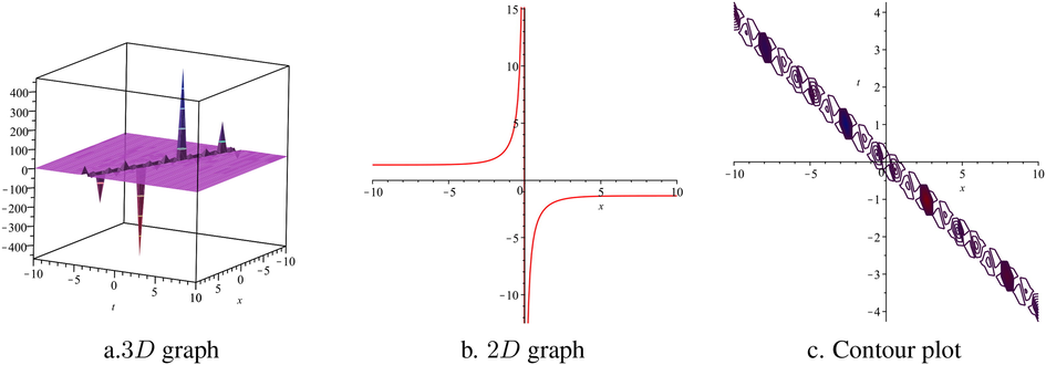
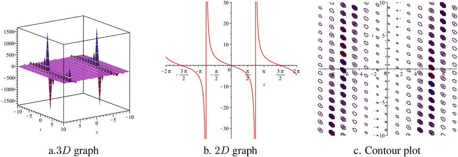
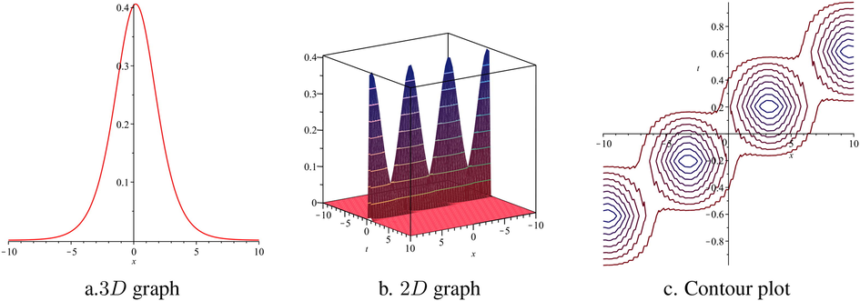
Figs. 1–5
manifest two of the answers under
and the contour plot surfaces by applying Maple.
Graphical representation of
for
and
within the interval
and
for two dimensional.
Graphical representation of
for
and
within the interval
and
for two dimensional.
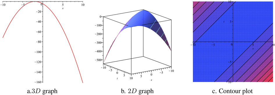
Graphical representation of
for
and
within the interval
and
for two dimensional.
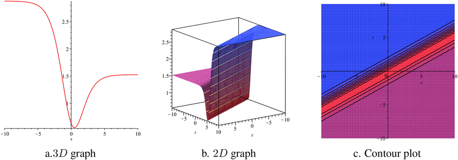
Graphical representation of
for
and
within the interval
and
for two dimensional.
Graphical representation of
for
and
within the interval
and
for two dimensional.
4 The (2 + 1)-dimensional Kadomtsev-Petviashvili equation
In this section, the method is utilised to obtain compaction, cuspon, kink, periodic, soliton traveling wave solution, singular soliton traveling wave solution and various kinds of solutions for the
-dimensional KP equation which are fundamental nonlinear evolution equations in the field of nonlinear dynamics. We consider the
-dimensional KP equation:
Applying
provides the Eq. (20) into a nonlinear ODE:
It is taken upon integrating twice and putting coefficients of integration to zeros. Making the homogeneous rule in Eq. (21), we obtain
and the solution as follows:
-
The first set: , where and E are free constants.
-
The second set: , where and E are free constants.
-
The third set: , where and E are free constants.
-
The fourth set: , where and E are free constants.
-
The fifth set: , where and E are free constants.
-
The sixth set: , where , and E are free constants.
-
The seventh set: , where , and E are free constants.
By putting the values of the first set including Eq. (8) into Eq. (22) and simplifying, leads to the following exact wave solutions: where .
Similarly for the second set, we have: where .
Similarly again for the third set, we find: where .
Similarly for the fourth set, we get: where .
Similarly for the fifth set, we obtain: where .
Similarly for the sixth set, we obtain: where .
Similarly for the seventh set, we obtain: where .
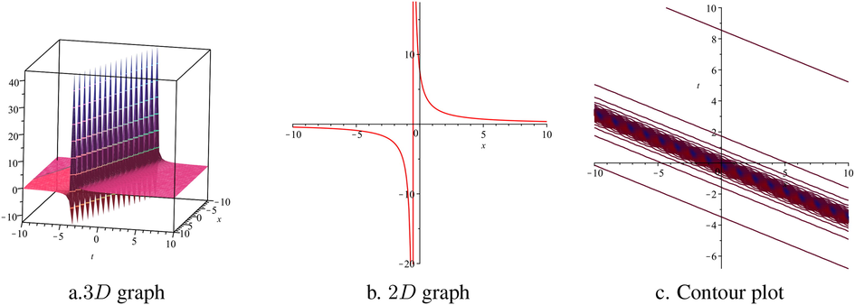
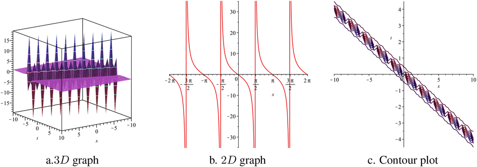
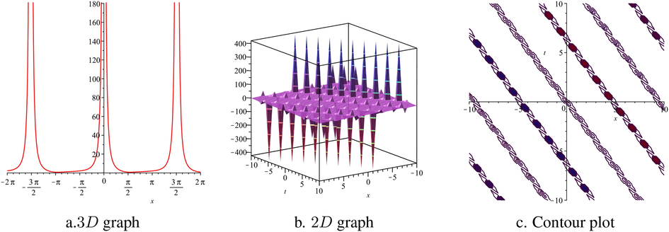
4.1 Graphical representations
We have successfully obtained sixty-three exact wave solutions in terms of some free unknown constants of the studied equation through the novel generalized
-expansion scheme. The obtained exact wave solutions are performed of rational, trigonometric and hyperbolic functions. If we change the appropriate values of the free unknown constants in each exact wave solutions, and next the solitary wave answers with compaction, cuspon, kink, periodic, soliton traveling wave solution, singular soliton traveling wave solution and various varieties of solutions may be succeeded. We have outlined some graphical illustration with
and the contour plot of the solitary wave answers by plugging the appropriate values of the free unknown constants. For more further assistance, the graphical depictions of
and
of studied equation are shown in Figs. 6–10
, respectively.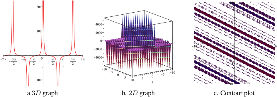
Graphical representation of
for
, and
within the interval
and
for two dimensional.
Graphical representation of
for
, and
within the interval
and
for two dimensional.
Graphical representation of
for
, and
within the interval
and
for two dimensional.
Graphical representation of
for
, and
within the interval
and
for two dimensional.
Graphical representation of
for
, and
within the interval
and
for two dimensional.
5 Results and discussion
Wazwaz (Wazwaz, 2007c) solved the KP equation and received only eight wave solutions through the tanh-coth method. Contrary, in the current paper by plugging the novel generalized -expansion process, numerous novel exact wave answers of the KP equation are constructed and also investigated three classes of explicit exact wave answers, for example, the hyperbolic, trigonometric and rational solutions under some unknown parameters. Comparing with Wazwaz (Wazwaz, 2007c) with our answers, we mentioned that (Wazwaz, 2007c) determined only trigonometric and hyperbolic types of solutions, but (Wazwaz, 2007c) did not solve any rational kind of solutions to the studied equation. On the contrary, we have determined rational, trigonometric and hyperbolic types of solutions to the considered equation. From the observation with (Wazwaz, 2007c), all of the solutions are achieved in this paper are new and has not been seen in the earlier literature. We also mentioned that compaction, cuspon, bell shape soliton, kink, periodic, soliton, bright periodic wave, dark periodic wave and various varieties of soliton of the considered equation are achieved through the studied method which is shown in Figs. 6–10 , respectively. These obtained solutions are the innovation and fulfilment of the present paper. We mention that few exact wave answers in the immediate investigation have a well-known physical application, like a liquid under small bubbles as well as turbulence (Fan et al., 2001), nonlinear wave models of fluid during an elastic tube as well as the acoustic dust waves within dusty plasmas under non-adiabatic dust charge fluctuation (Xue, 2003).
We actively investigated the novel generalized – expansion technique for ascertaining exact wave solutions of the KD and KP equations. The distinct variety of solitary wave answers such as compaction, bell shape soliton, cuspon, kink, periodic, soliton, bright periodic wave, dark periodic wave and various varieties of soliton are gained which implement in diverse fields of mathematical physics including fluid mechanics, nonlinear optics, quantum field theory, complex scalar nucleon field, and plasma physics. As our expected results, it may conclude that the investigated procedure is robust, sincere, and essential in giving numerous newly exact wave solutions of the different nonlinear wave shapes of PDEs. Subsequently, we would continue in our prospective studies.
Acknowledgment
The authors would like to acknowledge CAS-TWAS presidents fellowship program. The authors of this paper would like to express their sincere appreciation to the dear anonymous editor and referees for their valuable comments and suggestions which have led to an improvement in the presentation of the paper.
Declaration of Competing Interest
The authors declare that they have no known competing financial interests or personal relationships that could have appeared to influence the work reported in this paper.
References
- Application of the novel ( )-expansion method to traveling wave solutions for the positive Gardner-KP equation. Indian J. Pure Appl. Math.. 2016;47(1):85-96.
- [Google Scholar]
- Constructions of the optical solitons and others soliton to the conformable fractional Zakharov-Kuznetsov equation with power law nonlinearity. J. Taibah Univ. Sci.. 2020;14(1):94-100.
- [Google Scholar]
- The new solitary wave structures for the (2+1)-dimensional time-fractional Schrodinger equation and the space-time nonlinear conformable fractional Bogoyavlenskii equations. Alex. Eng. J.. 2020;59:2221-2232.
- [Google Scholar]
- Alam, M.N., Tunç, C., 2020c. Soliton solutions to the LWME in a MEECR and DSWE of soliton and multiple soliton solutions to the longitudinal wave motion equation in a magneto-electro elastic circular rod and the Drinfeld-Sokolov-Wilson equation. Miskolc Math. Notes. (in press).
- New solitary wave structures to the time fractional biological population. J. Math. Anal.. 2020;11(3):59-70.
- [Google Scholar]
- Exact solutions to the foam drainage equation by using the new generalized ( )-expansion method. Results Phys.. 2015;5:168-177.
- [Google Scholar]
- A novel -expansion method for solving the (3+1)-dimensional modified KdV-Zakharov-Kuznetsov equation in mathematical physics. Int. J. Comput. Sci. Math.. 2014;6(4):404-415.
- [Google Scholar]
- Exact traveling wave solutions of the (3+1)-dimensional mKdV-ZK equation and the -dimensional compound KdVB equation using new approach of the generalized -expansion method. Pramana J. Phys.. 2014;83(3):317-329.
- [Google Scholar]
- A novel -expansion method and its application to the Boussinesq equation. Chin. Phys. B. 2014;23(2) 020203
- [Google Scholar]
- Microtubules nonlinear models dynamics investigations through the -expansion method implementation. Mathematics. 2016;4:6.
- [Google Scholar]
- Exact traveling wave solutions to higher order nonlinear equations. J. Ocean Eng. Sci.. 2019;4(3):276-288.
- [Google Scholar]
- An analytical method for solving exact solutions of the nonlinear Bogoyavlenskii equation and the nonlinear diffusive predator-prey system. Alexandria Eng. J.. 2016;55:1855-1865.
- [Google Scholar]
- Shapes and dynamics of dual-mode Hirota-Satsuma coupled KdV equations: Exact traveling wave solutions and analysis. Chin. J. Phys.. 2019;58:49-56.
- [Google Scholar]
- A modified approach for a reliable study of new nonlinear equation: two-mode Korteweg-de Vries-Burgers equation. Nonlinear Dynam.. 2018;91(3):1619-1626.
- [Google Scholar]
- Exponential prototype structure for -dimensional Boiti–Leon–Pempinelli systems in mathematical physics. Waves Random Complex Media. 2016;26(2):189-196.
- [Google Scholar]
- On the new soliton and optical wave structures to some nonlinear evolution equations. Eur. Phys. J. Plus. 2017;132(11):459.
- [Google Scholar]
- Complex acoustic gravity wave behaviors to some mathematical models arising in fluid dynamics and nonlinear dispersive media. Opt. Quant. Electron.. 2018;50(1):19.
- [Google Scholar]
- Chen, G., Xin, X., Liu, H., 2019. The improved -expansion method and new exact solutions of nonlinear evolution equations in mathematical physics. Nonlinear Dyn. Article ID 4354310, 8 pages.
- Chen, J., Ma, Z., Hu, Y., 2018. Nonlocal symmetry, Darboux transformation and soliton–cnoidal wave interaction solution for the shallow water wave equation. J. Math. Anal. Appl. 460, 987–1003.
- A new complex line soliton for the two-dimensional KdV-Burgers equation. Phys. Lett. A. 2001;291:376-380.
- [Google Scholar]
- Exact solutions for a Dirac-type equation with N-fold Darboux transformation. J. Appl. Anal. Comput.. 2019;9(1):200-210.
- [Google Scholar]
- Symbolic methods to construct exact solutions of nonlinear partial differential equations. Math. Comput. Simul.. 1997;43(1):13-27.
- [Google Scholar]
- On the stability of solitary waves in weakly dispersive media. Sov. Phys. Dokl.. 1970;15:539-541.
- [Google Scholar]
- Exact solutions of nonlinear evolution equations using the extended modified function method. Tbilisi Math. J.. 2019;12(3):109-119.
- [Google Scholar]
- A -dimensional generalized BKP-Boussinesq equation: Lie group approach. Results Phys.. 2019;13 102239
- [Google Scholar]
- Some new integrable nonlinear evolution equations in - dimensions. Phys. Lett. A. 1984;102(1–2):15-17.
- [Google Scholar]
- A new solitary wave solution for the new Hamiltonian amplitude equation. J. Phys. Soc. Jpn.. 2005;74:896-897.
- [Google Scholar]
- Exact solutions to Euler equation and Navier-Stokes equation. Angew. Math. Phys.. 2019;70:43.
- [Google Scholar]
- The singular manifold method and exact periodic wave solutions to a restricted BLP dispersive long wave system. Rep. Math. Phys.. 2005;56:367-378.
- [Google Scholar]
- Exact travelling wave solutions to the (3+1)D Kadomtsev-Petviashvili equation. Acta Physica Pol.. 2005;108:421-428.
- [Google Scholar]
- Analytical research of -dimensional Rossby waves with dissipation effect in cylindrical coordinate based on Lie symmetry approach. Adv. Differ. Equ.. 2019;2019(1):13.
- [Google Scholar]
- Solution of different geometries reflected reactors neutron diffusion equation using the homotopy perturbation method. Res. Phys.. 2019;12:61-66.
- [Google Scholar]
- Exact traveling wave solutions of nonlinear evolution equations: indeterminant homogeneous balance and linearizability. Math. Stat.. 2019;7(1):10-13.
- [Google Scholar]
- New exact solutions for Konopelchenko-Dubrovsky equation using an extended Riccati equation rational expansion method. Commun. Theor. Phys.. 2006;45(5):769-776.
- [Google Scholar]
- Syam, M.I., 2019. The solution of Cahn-Allen equation based on Bernoulli sub-equation method. Results Phys. 514, 102413.
- Exact travelling wave solutions for Konopelchenko-Dubrovsky equation by the first integral method. Appl. Appl. Math.: Int. J.. 2011;6(1):153-161.
- [Google Scholar]
- Exact solutions of the unstable nonlinear Schrödinger equation with the new Jacobi elliptic function rational expansion method and the exponential rational function method. Optik-Int. J. Light Electron Opt.. 2016;127(23):11124-11130.
- [Google Scholar]
- New compactons, solitons and periodic solutions for nonlinear variants of the KdV and the KP equations. Chaos Solitons Fractals. 2004;22(1):249-260.
- [Google Scholar]
- New kinks and solitons solutions to the -dimensional Konopelchenko-Dubrovsky equation. Math. Comput. Modell.. 2007;45:473-479.
- [Google Scholar]
- Travelling wave solutions to (2+1)-dimensional nonlinear evolution equations. J. Nat. Sci. Math.. 2007;1:113.
- [Google Scholar]
- Traveling wave solutions to (2+1)-dimensional nonlinear evolution equations. J. Nat. Sci. Math.. 2007;1:1-13.
- [Google Scholar]
- Multiple-soliton solutions for a (3+1)-dimensional generalized KP equation. Commun. Nonlinear Sci. Numer. Simul.. 2012;17:491-495.
- [Google Scholar]
- Solving the -dimensional KP-Boussinesq and BKP-Boussinesq equations by the simplified Hirota’s method. Nonlinear Dyn.. 2017;88:3017-3021.
- [Google Scholar]
- Kadomtsev-Petviashvili (KP) Burgers equation in a dusty plasmas with non-adiabatic dust charge fluctuation. Eur. Phys. J. D. 2003;26:211-214.
- [Google Scholar]


