

Translate this page into:
New preconditioning and half-sweep accelerated overrelaxation solution for fractional differential equation
⁎Corresponding authors at: Anand International College of Engineering, Agra Road, Jaipur, Rajasthan 303012, India (P. Agarwal); Tadris Matematika, UIN Fatmawati Sukarno Bengkulu, Bengkulu 38211, Indonesia. goyal.praveen2011@gmail.com (Praveen Agarwal), andang99@gmail.com (Andang Sunarto),
-
Received: ,
Accepted: ,
This article was originally published by Elsevier and was migrated to Scientific Scholar after the change of Publisher.
Peer review under responsibility of King Saud University.
Abstract
The present paper investigates the approximate solution of a one-dimensional linear space-fractional diffusion equation using a new preconditioning matrix to develop an efficient half-sweep accelerated overrelaxation iterative method. The proposed method utilizes unconditionally stable implicit finite difference schemes to formulate the discrete approximation equation to the problem. The formulation employs the Caputo fractional derivative to treat the space-fractional derivative in the problem. The paper's focus is to assess the improvement in terms of the convergence rate of the solution obtained by the proposed iterative method. The numerical experiment illustrates the superiority of the proposed method in terms of solution efficiency against one of the existing preconditioned methods, preconditioned accelerated overrelaxation and implicit Euler method. The proposed method reveals the ability to compute the solution with lesser iterations and faster computation time than the preconditioned accelerated overrelaxation and implicit Euler method. The method introduced in the paper, half-sweep preconditioned accelerated overrelaxation, has the potential to solve a variety of space-fractional diffusion models efficiently. Future investigation will improve the absolute errors of the solutions.
Keywords
Finite difference method
Caputo fractional derivative
Space-fractional derivative
Half-sweep
Preconditioning matrix
Accelerated overrelaxation

1 Introduction
Fractional calculus has gained considerable popularity and importance for almost five decades now. It is mainly from various demonstrated applications in biological science, physical science and other branches of sciences. Fractional calculus has significantly contributed to the modelling of transmission of Covid-19 infection (Cui and Liu, 2022), pharmacokinetic compartments (Azizi, 2022), Meningitis with treatment and vaccination (Peter et al., 2022), tumour and immune cells interactions (Tang et al., 2022), mechanical behaviour of asphalt mastic (Lagos-Varas et al., 2022), fluid flow and heat transfer (Turkyilmazoglu, 2022), control behaviour of wearable exoskeletons (Sun et al., 2021) and control behaviour of a knee joint orthosis (Delavari and Jokar, 2021). Many different fractional differential equations (FDE) have arisen from the realistic applications of fractional calculus. FDE is a generalization of differential equations based on the established theory and application of fractional calculus. FDE can also be considered the extended partial differential equations by modifying the integer-order derivative into the fractional-order derivative.
The solutions of FDEs must be obtained to understand the fractional mathematical models. Various solution methods have been proposed to the literature, such as the finite difference method with collocation (Mesgarani et al., 2021;Safdari et al., 2020;Jaleb and Adibi, 2019), finite difference method with preconditioners (Barakitis et al., 2022; Shao and Kang, 2022; Sunarto et al., 2022; Sunarto et al., 2021), finite difference method with Lucas polynomials (Ali et al., 2022), Adomian decomposition method (Turkyilmazoglu, 2022; Ahmad et al., 2022; Turkyilmazoglu, 2021) and variational iteration method (Ibraheem et al., 2022). Following the high interest towards the finite difference method with preconditioners, this paper aims to investigate the approximate solution of a type of FDE, the space-fractional diffusion equation, using a new preconditioning matrix to develop an efficient half-sweep accelerated overrelaxation iterative method. This paper utilizes the Caputo fractional derivative to treat the space-fractional derivative because it allows the inclusion of traditional and conventional initial-boundary conditions in the formulation of the problem (Elsayed and Orlov, 2020). In addition, the Caputo space-fractional derivative's memories affect the dynamics of the considered variables (Sene, 2022). The importance of Caputo space-fractional can be seen in the modelling of biological models (Haghi and Ghanbari, 2022), sediment suspension in ice-covered channels (Wang et al., 2022), drug diffusion through the skin (Caputo and Cametti, 2021) and chaotic processes (Owolabi et al., 2020).
The paper's focus is to assess the improvement in terms of the convergence rate of the solution obtained by the proposed iterative method. Among various iterative methods that can be used to solve the generated system of equations from an FDE (She et al., 2023; AllaHamou et al., 2022; Wen et al., 2022; Sun et al., 2022; Tang and Huang, 2022), the paper proposes a modified accelerated overrelaxation iterative method using a new preconditioning matrix with a half-sweep iteration strategy. The paper's contribution is a new preconditioned iterative method that can solve a space-fractional diffusion equation at a good efficiency level. The following sections of the paper are organized: Section 2 formula tesa discrete approximation to a one-dimensional linear space-fractional diffusion equation using a half-sweep type finite difference method in the Caputo sense. Section 3 derives the proposed iterative method to solve the generated system of equations from the discretized problem. Section 4 illustrates the numerical results of solving several initial-boundary value problems using the proposed numerical method and the comparison analysis against the standard preconditioned accelerated overrelaxation method (Sunarto et al., 2016). The conclusion of the paper is stated in Section 5.
2 Half-sweep type finite difference method in caputosense
This section describes the formulation of a discrete approximation to a one-dimensional linear space-fractional diffusion equation using a half-sweep type finite difference method in the Caputo sense. The paper usesa general space fractional FDE in the formulation, which is given by (Reutskiy and Lin, 2018),
Based on Eq. (1), the variables , and 3 are either constants or functions in terms of while is a source function.
This paper utilizes half-sweep type implicit finite difference schemes to discretize Eq. (1) for the time derivative, integer-order space derivative and other functions (Ibrahim and Abdullah, 1995; Sunarto et al., 2021; Chew et al., 2021). Meanwhile, Caputo fractional derivative is applied to approximate the fractional-order space derivative. Below is the following established definition of Caputo fractional derivative used in the discretization (Oldham and Spanier, 2006):
Definition 1. Let
be the upper limit of the integral, and a real number
be the fractional order, such that
where
is a positive integer. Then,
represents the
-th order derivative of a smooth function
. Hence, the Caputo fractional derivative of
is defined as
Combining half-sweep type finite difference schemes and Eq. (3) gives the following discrete approximation to the space-fractional derivative,
Then, putting Eq. (5) together with the half-sweep finite differences for other derivatives such as first-order time derivative, first-order space derivative and source functions, Eq. (1) can be rewritten in the form of finite difference approximation equation in Caputo sense as follows,
Based on Eq. (9), one may have the following equations subject to different values of
. For instance, when
, Eq. (9) becomes
Hence, when the pattern continues for
, one can easily obtain a general form of the equation that can generate a large-scale system of equations as follows,
When Eq. (12) takes all points bounded by a specified solution domain, the large-scale system of equations can be expressed in the form of a matrix equation,
Noted that the matrix dimensions of matrix , and are , , and , respectively. This paper suggests that an efficient iterative method needs to be developed to solve a complex matrix equation like Eq. (20). Hence, this paper proposes a new preconditioning matrix that can enhance the convergence rate of the iterated solutions. Moreover, this paper develops a new iterative method called the half-sweep preconditioned accelerated overrelaxation.
3 Derivation of a preconditioned iterative method
This section is devoted to showing the derivation of the proposed preconditioned iterative method to solve the system of equations shown (Eq. (20)). From here, the paper shall use HSPAOR to stand for the proposed method to solve space-fractional diffusion problems. To begin the derivation, let's consider a transformed matrix equation that corresponds to Eq. (20) as follows,
Eq. (24) is obtained using the following matrix transformations with a new preconditioning matrix
,
Based on the coefficient matrix
that presents in the transformed matrix equation shown in Eq. (24), this paper considers a unique decomposition of matrix
that is given by
Hence, to achieve the desired convergence rate and the objective of the numerical study, which is to investigate the numerical solutions, a manual selection of accelerating parameters is conducted by running the developed simulation program several times until the smallest number of iterations is obtained. The selection procedure can be described as follows. We initially let and use different values of within the range . When the smallest number of iterations is obtained for some value of , by using the “optimum” value of , we increase the value of gradually until the final smallest number of iterations is obtained. The implementation of the HSPAOR method is programmed using the C++ programming language. The structure of the code and instructions are made thoroughly. Due to the copyright issue, the paper can only provide the following algorithm.
Algorithm 1: HSPAOR method to solve space-fractional diffusion equations
-
Set the initial guess and the tolerance error
-
For , iterate Eq. (31).
-
For , run linear interpolation module.
-
If then go to the next time-step or .
-
If the time-step reaches the final step or , display outputs such as numerical solutions, the maximum number of iterations, program execution time, and maximum absolute errors.
4 Numerical experiment and results
Section 4 illustrates the proposed method's results by solving several initial-boundary value problems of space-fractional diffusion. Below are the following test problems considered in this paper.
Consider the given one-dimensional linear time-dependent space-fractional diffusion equation (Khader, 2011),
Based on Eq. (32), the value of
represents the diffusion coefficient, while the function
is the source of diffusion. The accuracy of the numerical solution obtained by HSPAOR is compared to the exact solution,
Consider another one-dimensional linear time-dependent space-fractional diffusion equation (Khader, 2011),
Based on Eq. (32),
represents the diffusion coefficient, while
is the source function. The accuracy of the numerical solution obtained by HSPAOR is compared to the exact solution,
The results considered take account of numerical solutions, the number of iterations to obtain the final solutions
, the final time after completing the C++ program,which is measured in seconds
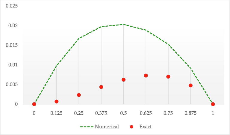
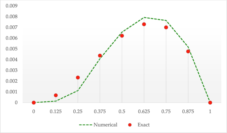
and the value of absolute errors. Fig. 1 until 6 show the numerical solutions obtained by HSPAOR after solving Examples 1 and 2 using
and
. The solutions are compared to the exact solutions at various points and time level
seconds.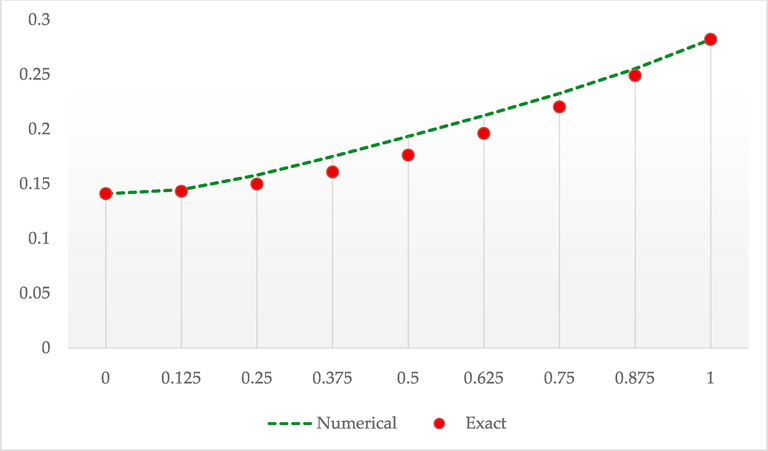
Numerical solutions by HSPAOR against exact solutions of Example 1 at
.
Based on Figs. 1 through 3, the effectiveness of HSPAOR in computing numerical solutions of Example 1 at various orders of space-fractional is illustrated. The numerical solutions are sufficiently close to the provided exact solutions at
and well-fitted to the exact solutions at both
and
. However, HSPAOR shows some disadvantages in computing the numerical solutions of Example 2 at
and
compared to the exact solutions, see Figs. 4 and 5. The accuracy of the solutions by HSPAOR is better when the value of space-fractional order is set to be greater than 1.5 or
for instance, see Fig. 6.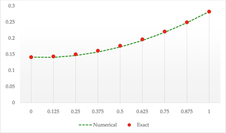
Numerical solutions by HSPAOR against exact solutions of Example 1 at
.
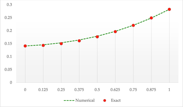
Numerical solutions by HSPAOR against exact solutions of Example 1 at
.
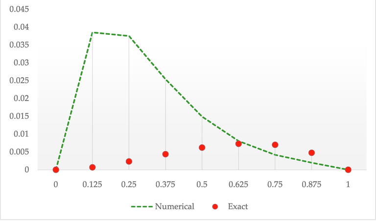
Numerical solutions by HSPAOR against exact solutions of Example 2 at
.
Numerical solutions by HSPAOR against exact solutions of Example 2 at
.
Numerical solutions by HSPAOR against exact solutions of Example 2 at
.
Next, comparison in terms of the number of iterations, program completion time and maximum absolute error between HSPAOR and two tested methods, such as the standard or full-sweep preconditioned accelerated overrelaxation (FSPAOR) (Sunarto et al., 2016) and implicit Euler (Meerschaert and Tadjeran, 2006) is shown in Tables 1 until 6. The comparison is conducted using three different values of space-fractional order,
, and
, and five different numbers of domain points for the consistency of the solutions.
Method
Seconds
Max Error
128
Implicit Euler
74
1.48
2.37e-02
FSPAOR
33
0.73
2.37e-02
HSPAOR
19
0.30
2.24e-02
256
Implicit Euler
152
11.64
2.44e-02
FSPAOR
64
5.21
2.44e-02
HSPAOR
35
2.73
2.37e-02
512
Implicit Euler
312
90.64
2.47e-02
FSPAOR
127
35.22
2.47e-02
HSPAOR
70
15.21
2.44e-02
1024
Implicit Euler
709
972.27
2.49e-02
FSPAOR
272
342.76
2.49e-02
HSPAOR
147
139.66
2.47e-02
2048
Implicit Euler
1647
3727.45
2.52e-02
FSPAOR
597
1195.59
2.52e-02
HSPAOR
318
452.46
2.49e-02
Based on Tables 1 until 6, the comparison results show that the HSPAOR method is more efficient than he FSPAOR and implicit Euler methods in solving Examples 1 and 2. The number of iterations and program completion time required by the HSPAOR method to obtain the final numerical solutions at all different points are significantly lesser than the other two tested methods. However, the absolute errors produced by the HSPAOR method are slightly larger than the FSPAOR and implicit Euler methods for Example 1 using
and
and Example 2 using
. Furthermore, by observing the consistency of the numerical solutions with the increasing number of points in computation, this paper found that the absolute errors show some sign of gradual growth for Example 1 at
and Example 2 at all values of
.
Method
Seconds
Max Error
128
Implicit Euler
251
4.95
6.21e-04
FSPAOR
77
1.84
6.21e-04
HSPAOR
40
0.61
6.99e-04
256
Implicit Euler
666
51.01
5.69e-04
FSPAOR
204
17.51
5.69e-04
HSPAOR
100
7.040
6.21e-04
512
Implicit Euler
1780
550.52
5.35e-04
FSPAOR
548
177.13
5.35e-04
HSPAOR
261
49.26
5.69e-04
1024
Implicit Euler
4750
2970.31
5.13e-04
FSPAOR
1469
873.87
5.13e-04
HSPAOR
696
523.33
5.35e-04
2048
Implicit Euler
13,230
15348.70
5.09e-04
FSPAOR
4012
4274.43
5.09e-04
HSPAOR
1856
2132.82
5.24e-04
Method
Seconds
Max Error
128
Implicit Euler
930
18.29
3.99e-04
FSPAOR
234
5.56
3.99e-04
HSPAOR
103
2.43
4.03e-04
256
Implicit Euler
3029
233.01
3.97e-04
FSPAOR
769
66.34
3.97e-04
HSPAOR
323
26.16
3.99e-04
512
Implicit Euler
9840
2755.31
3.96e-04
FSPAOR
2528
828.27
3.96e-04
HSPAOR
1067
305.81
3.97e-04
1024
Implicit Euler
46,847
7259.97
3.95e-04
FSPAOR
11,783
2081.94
3.95e-04
HSPAOR
5463
1005.63
3.96e-04
2048
Implicit Euler
187,322
28979.20
3.93e-04
FSPAOR
47,253
8800.61
3.93e-04
HSPAOR
22,125
4232.91
3.95e-04
Method
Seconds
Max Error
128
Implicit Euler
57
1.42
5.44e-02
FSPAOR
33
0.73
5.44e-02
HSPAOR
19
0.30
5.16e-02
256
Implicit Euler
117
10.95
5.58e-02
FSPAOR
64
5.21
5.58e-02
HSPAOR
35
2.73
5.44e-02
512
Implicit Euler
249
81.84
5.58e-02
FSPAOR
127
35.22
5.58e-02
HSPAOR
70
15.21
5.28e-02
1024
Implicit Euler
560
853.89
5.65e-02
FSPAOR
272
342.76
5.65e-02
HSPAOR
147
139.66
5.32e-02
2048
Implicit Euler
1296
3157.00
5.80e-02
FSPAOR
597
1195.59
5.80e-02
HSPAOR
318
452.46
5.73e-02
Method
Seconds
Max Error
128
Implicit Euler
182
4.41
1.80e-02
FSPAOR
77
1.84
1.80e-02
HSPAOR
40
0.61
1.73e-02
256
Implicit Euler
481
45.32
1.84e-02
FSPAOR
204
17.51
1.84e-02
HSPAOR
100
7.04
1.81e-02
512
Implicit Euler
1297
484.4
2.39e-02
FSPAOR
548
177.13
2.39e-02
HSPAOR
261
49.26
1.84e-02
1024
Implicit Euler
3493
2614.51
2.45e-02
FSPAOR
1469
873.87
2.45e-02
HSPAOR
696
523.33
1.86e-02
2048
Implicit Euler
9541
13859.30
2.92e-02
FSPAOR
4012
4274.43
2.92e-02
HSPAOR
1856
2132.82
1.86e-02
Method
Seconds
Max Error
128
Implicit Euler
569
13.7
1.25e-04
FSPAOR
234
5.56
1.25e-04
HSPAOR
103
2.43
1.76e-04
256
Implicit Euler
1861
164.77
1.44e-04
FSPAOR
769
66.34
1.44e-04
HSPAOR
323
26.16
1.76e-04
512
Implicit Euler
6235
2027
1.53e-04
FSPAOR
2528
828.27
1.53e-04
HSPAOR
1067
305.81
1.82e-04
1024
Implicit Euler
29,937
5248.83
1.65e-04
FSPAOR
11,783
2081.94
1.65e-04
HSPAOR
5463
1005.63
1.84e-04
2048
Implicit Euler
121,482
22345.00
2.30e-04
FSPAOR
47,253
8800.61
2.30e-04
HSPAOR
22,125
4232.91
2.45e-04
To complete the numerical experiment, this paper compares the maximum absolute errors produced by the proposed HSPAOR method (with a time-step 0.2) with some numerical methods, including the methods that utilize the Chebyshev polynomial of degree
. The error comparison is made using a similar setting of Example 2 that has been done (Khader, 2011; Saadatmandi and Dehghan, 2011; Azizi and Loghmani, 2013). Table 7 shows the comparison in terms of maximum absolute errors against the selected three methods.
HSPAOR
(Khader, 2011),
(Saadatmandi and Dehghan, 2011)
(Azizi and Loghmani, 2013),
0
0
1.71e-04
0
0
0.1
5.87e-03
2.11e-05
2.89e-05
1.40e-07
0.2
6.98e-03
1.77e-04
1.09e-04
9.06e-07
0.3
6.31e-03
3.01e-04
2.20e-04
3.25e-08
0.4
5.10e-03
4.04e-04
3.40e-04
6.55e-08
0.5
3.83e-03
4.89e-04
4.45e-04
1.02e-08
0.6
2.67e-03
5.63e-04
5.15e-04
7.38e-09
0.7
1.71e-03
6.33e-04
5.27e-04
1.64e-07
0.8
9.54e-04
7.06e-04
4.60e-04
2.75e-08
0.9
3.91e-04
7.87e-04
2.91e-04
1.32e-07
1.0
0
8.83e-04
0
0
Based on the findings through the numerical experiment, HSPAOR possesses the advantage in terms of computational efficiency, especially when a large system of equations is considered. The reason is that the iteration procedure by the preconditioned accelerated overrelaxation is highly efficient in computing the generated system of equations. Besides that, using a half-sweep strategy in formulating the finite difference approximation in the Caputo sense has successfully reduced the computational complexity in the developed program. However, to achieve a greater efficiency level, the accuracy of the solution becomes the trade-off. The disadvantage of the HSPAOR method is revealed when it is used to solve Example 2 using and . Since the development of HSPAOR is based on implicit finite difference schemes, the accuracy of HSPAOR is limited by the properties of implicit finite difference schemes, which are second-order accurate in space. This paper hypothesized that the magnitude of absolute errors could be reduced using higher-order finite difference schemes and different fractional definitions.
5 Conclusion
This paper successfully developed an efficient half-sweep accelerated overrelaxation iterative method using a new preconditioning matrix to solve several space-fractional diffusion problems. The Caputo fractional derivative is compatible with formulating a discrete approximation equation via implicit finite difference schemes. The numerical results showed the superiority of the proposed method in terms of solution efficiency against the standard preconditioned accelerated overrelaxation and implicit Euler methods. When the absolute errors by the proposed method are compared against several existing numerical methods, the errors are slightly larger than all considered methods. The magnitude of errors can be reduced by using higher-order finite difference schemes and different fractional definitions. Based on the performance of the proposed method in terms of efficiency, it has the potential to solve a variety of space-fractional diffusion models efficiently. Future investigation will improve the solutions' absolute errors so that the proposed method's reliability can be increased.
Acknowledgment
NBHM (DAE). Grant Number: 02011/12/2020 NBHM (R.P)/RD II/7867.
Ministry of Science and High Education of the Russian Federation and the Peoples' Friendship University of Russia. Grant Number: 075-15-2021-603
Declaration of Competing Interest
The authors declare that they have no known competing financial interests or personal relationships that could have appeared to influence the work reported in this paper.
References
- Analytical solution of one dimensional time fractional black-scholes equation through laplaceadomian decomposition method. Mathe. Eng., Sci. Aerospace.. 2022;13(2):373-386.
- [Google Scholar]
- Numerical solution of one- and two-dimensional time-fractional burgers equation via lucas polynomials coupled with finite difference method. Alex. Eng. J.. 2022;61(8):6077-6087.
- [CrossRef] [Google Scholar]
- Monotone iterative technique for solving finite difference systems of time fractional parabolic equations with initial/periodic conditions. Appl. Numer. Math.. 2022;181:561-593.
- [CrossRef] [Google Scholar]
- Numerical approximation for space-fractional diffusion equationsvia Chebyshev finite difference method. J. Fractional Appl.. 2013;4(2):303-311.
- [Google Scholar]
- Application of the fractional calculus in pharmacokinetic compartmental modeling. Commun. Biomathe. Sci.. 2022;5(1):63-77.
- [CrossRef] [Google Scholar]
- Preconditioners for fractional diffusion equations based on the spectral symbol. Num. Linear Algebra Appl.. 2022;29(5) Article ID e2441
- [CrossRef] [Google Scholar]
- Diffusion through skin in the light of a fractional derivative approach: Progress and challenges. J. Pharmacokinet Pharmacodyn.. 2021;48:3-19.
- [CrossRef] [Google Scholar]
- Solving one-dimensional porous medium equation using unconditionally stable half-sweep finite difference and SOR method. Mathe. Stat.. 2021;9(2):166-171.
- [CrossRef] [Google Scholar]
- Modeling the transmission phenomena of covid-19 infection with the effect of vaccination via noninteger derivative under real statistic. Fractals.. 2022;30(5) Article ID 2240152
- [CrossRef] [Google Scholar]
- Intelligent fractional-order active fault-tolerant sliding mode controller for a knee joint orthosis. J. Intell. Robotic Syst.: Theory Appl.. 2021;102 Article ID 39
- [CrossRef] [Google Scholar]
- Numerical scheme for solving time-space vibration string equation of fractional derivative. Mathematics. 2020;8 Article ID 1069
- [CrossRef] [Google Scholar]
- Existence and properties of positive solutions for Caputo fractional difference equation and applications. Computational Methods for. Diff. Eqs.. 2022;10(3):567-579.
- [CrossRef] [Google Scholar]
- Novel approximate solution for fractional differential equations by the optimal variational iteration method. J. Comput. Sci.. 2022;64 Article ID 101841
- [CrossRef] [Google Scholar]
- Solving the two dimensional diffusion equation by the fourpoint explicit decoupled group (EDG) iterative method. Int. J. Comput. Mathe.. 1995;58(3–4):253-263.
- [CrossRef] [Google Scholar]
- On a novel modification of the Legendre collocation method for solvingfractional diffusion equation. Comput. Methods Diff. Eqs.. 2019;7:480-496.
- [Google Scholar]
- On the numerical solutions for the fractional diffusion equation. Commun. Nonlinear Sci. Numer. Simul.. 2011;16(6):2535-2542.
- [CrossRef] [Google Scholar]
- Viscoelasticity modelling of asphalt mastics under permanent deformation through the use of fractional calculus. Constr. Build. Mater.. 2022;329 Article ID 127102
- [CrossRef] [Google Scholar]
- Finite difference approximations for two-sided space-fractional partial differential equations. Appl. Numer. Math.. 2006;56(1):80-90.
- [CrossRef] [Google Scholar]
- Numerical treatment of the spacefractional advection–dispersion model arising in groundwater hydrology. Comput. Appl. Mathe.. 2021;40 Article ID 22
- [CrossRef] [Google Scholar]
- The Fractional Calculus. New York: Dover Publications; 2006.
- Modelling of chaotic processes with Caputo fractional order derivative. Entropy. 2020;22(9) Article ID 1027
- [CrossRef] [Google Scholar]
- A mathematical model analysis of Meningitis with treatment and vaccination in fractional derivatives. Int. J. Appl. Comput. Math.. 2022;8 Article ID 117
- [CrossRef] [Google Scholar]
- A semi-analytic collocation method for space fractional parabolic PDE. Int. J. Comput. Mathe.. 2018;95(6–7):1326-1339.
- [CrossRef] [Google Scholar]
- A tau approach for solution of the space fractional diffusion equation. Comput. Math. Appl.. 2011;62(3):1135-1142.
- [CrossRef] [Google Scholar]
- Convergence analysis of the spacefractional-order diffusion equation based on the compact finite difference scheme. Comput. Appl. Mathe.. 2020;39 Article ID 62
- [CrossRef] [Google Scholar]
- Second-grade fluid with Newtonian heating under Caputo fractional derivative: analytical investigations via Laplace transforms. Mathe. Modell. Num. Simulat. Appl.. 2022;2(1):13-25.
- [CrossRef] [Google Scholar]
- A preconditioner based on sine transform for space fractional diffusion equations. Appl. Num. Mathe.. 2022;178:248-261.
- [CrossRef] [Google Scholar]
- An unconditionally convergent RSCSCS iteration method for riesz space fractional diffusion equations with variable coefficients. Math. Comput. Simul. 2023;203:633-646.
- [CrossRef] [Google Scholar]
- Existence of solutions to a class of fractional differential equations. J. Nonlinear Model. Anal.. 2022;4:409-442.
- [CrossRef] [Google Scholar]
- Model-free fractional-order adaptive back-stepping prescribed performance control for wearable exoskeletons. Int. J. Intell. Robot. Appl.. 2021;5:590-605.
- [CrossRef] [Google Scholar]
- Approximation solution of the fractional parabolic partial differential equation by the half-sweep and preconditioned relaxation. Symmetry. 2021;13(6) Article ID 1005
- [CrossRef] [Google Scholar]
- Application of the full-sweep AOR iteration conceptfor space-fractional diffusion equation. J. Phys. Conf. Ser.. 2016;710 Article ID 012019
- [Google Scholar]
- Numerical investigation on the solution of a space-fractional via preconditioned SOR iterative method. Progress Fractional Diff. Appl.. 2022;8(2):289-295.
- [CrossRef] [Google Scholar]
- A lopsided scaled DTS preconditioning method for the discrete space-fractional diffusion equations. Appl. Math. Lett.. 2022;131
- [CrossRef] [Google Scholar]
- Modeling the dynamics of tumor–immune cells interactions via fractional calculus. Eur. Phys. J. Plus.. 2022;137 Article ID 367
- [CrossRef] [Google Scholar]
- Nonlinear problems via a convergence accelerated decomposition method of adomian. CMES – Comput. Model. Eng. Sci.. 2021;127(1):1-22.
- [CrossRef] [Google Scholar]
- Transient and passage to steady state in fluid flow and heat transfer within fractional models. Int. J. Numer. Meth. Heat Fluid Flow 2022
- [CrossRef] [Google Scholar]
- Fractional derivative modeling for sediment suspension in ice-covered channels. Environ. Sci. Pollut. Res. 2022
- [CrossRef] [Google Scholar]
- Landweber iteration method for simultaneous inversion of the source term and initial data in a time-fractional diffusion equation. J. Appl. Math. Comput.. 2022;68:3219-3250.
- [CrossRef] [Google Scholar]


