

Translate this page into:
New exact solitary wave solutions, bifurcation analysis and first order conserved quantities of resonance nonlinear Schrödinger’s equation with Kerr law nonlinearity
⁎Corresponding author. gaowei@ynnu.edu.cn (Wei Gao)
-
Received: ,
Accepted: ,
This article was originally published by Elsevier and was migrated to Scientific Scholar after the change of Publisher.
Peer review under responsibility of King Saud University.
Abstract
This paper anatomizes the exact solutions of the resonant non-linear Schrödinger’s equation (R-NLSE) with the Kerr law non-linearity with the assistance of the new extended direct algebraic technique. The secured soliton erections are newfangled and unreservedly invigorating for investigators. The graphically comprehensive report of some specific solutions is embellished with the well-judged values of parameters to illustrate their propagation. Then a planer dynamical system is introduced and the bifurcation analysis has been executed to figure out the bifurcation structures of the non-linear and super non-linear traveling wave solutions of the heeded model. All possible phase portraits are exhibited with specific values of parameters. Furthermore, a precise class of non-trivial and first-order conserved quantities is enumerated by the intervention of the multiplier approach.
Keywords
Schrödinger’s equation
Bifurcation theory
Conservation laws

1 Introduction
The non-linear Schrödinger’s equation (NLSE) has an imperative influence and pivotal significance in different branches of science. Quantum mechanics, non-linear optics, fluid dynamics, and plasma physics are some of the fields where NLSE has appeared. The R-NLSE has availed oneself of the study of Madelung fluids and solitonic dynamics in various non-linear processes (Baleanua et al., 2017 and references therein):
The independent variables x and t depicts the non-dimensional distance in Eq. (1), along the fiber and temporal variables, respectively. The complex valued dependent variable represents wave profile, while, the constants parameters and are the coefficients of group-velocity dispersion, non-Kerr non-linearity and resonant non-linearity respectively. In the Eq. (1), real valued and n-times differentiable function is defined as: where the two-dimensional linear space of represents by Argand plane . Here we are assuming , which arises in water waves and the non-linear fiber optics when the refractive index is directly proportional to intensity (Biswas and Konat, 2006).
The R-NLSE equation has been discussed by many means in literature. Over the last few years, scientists have been quantified the exact solutions of Eq. (1) by utilizing numerous distinct approaches. The Jacobi elliptic tool has been exploited to quantifying the exact structures of Eq. (1) and also simplest equation approach took under consideration (Eslami et al., 2013). To extract the exact solitary wave solutions of Eq. (1), D. Baleanu has been prosecuted the Ricatti-Bernoulli sub-ODE technique (Baleanua et al., 2017). One of the aspirations of this exploration is to deliberate a futuristic class of exact solutions. On that account, a new direct extended algebraic approach is maneuvered to come across the exact solutions of Eq. (1). Some of the classical contributions on numerical aspects of the PDEs are reported in Cattani et al. (2013), Cattani et al. (2012), Heydari et al. (2015), Kumar et al. (2018), Kumar et al. (2020), Rushchitsky et al. (2004), Singh and Srivastava (2020), Singh (xxxxx), Singh (2020), Singh et al. (2019), Singh et al. (2020) and Yadav et al. (2019). In recent years, the study of differential equations employing bifurcation analysis is a hot topic of research. Dubinov et. al. in Dubinov et al. (2012) characterized a new class of nonlinear and super-nonlinear waves. In Zhang et al. (2013), a class of solutions is obtained for Klein–Gordon–Zakharov equations by using bifurcation theory. More recently, Sharma-Tasso-Olver equation is dealt with utilizing bifurcation theory (Ali et al., 2018) and the complete classification of waves is presented. By the best of our knowledge, any study related to the behavior of nonlinear and super-nonlinear traveling waves for R-NLSE equation is not done before. Consequently, a profundity anatomy of Eq. (1) along with these trajectories is fascinating and is propounded here.
Conservation laws have miraculous contributions to unfold the partial differential equations and in various applications. The suggestion about conservation laws ejaculated by the perception of physical laws like mass, energy, and momentum. Initially, The ideology and exploitation of the Noether’s theorem was authenticated by German mathematician Emmy Noether and also certified as a well-ordered approach for uncovering the conservation laws Bessel-Hagen, 1921. Noether theorem states that each Euler - Lagrange equation’s Noether symmetry corresponds to a difference equation’s conservation law. Noether’s theorem works only for a variational differential equation, yet there are differential equations which have no Lagrangian equations which can be dealt with different approaches available in the literature, some of them are (Anco and Bluman, 2002; Ibragimov, 2007; Kara and Mahomed, 2006) while computer package for construction of conserved quantities by using (Anco and Bluman, 2002) is also developed (Cheviakov, 2007) and utilized in this research. Here we search out the first order nontrivial conserved quantities of Eq. (1) by using a multiplier approach (Anco and Bluman, 2002). Some latest works related to exact solutions and conservation laws are given in Baskonus et al. (2019), Eskitaolu et al. (2019), Khalique et al. (2018), Khalique and Mhlanga (2018) and Moleleki et al. (2018).
This report is designated as segment 2 is customized for the exact solutions of Eq. (1) by using the new direct extended algebraic technique. Bifurcation analysis of Eq. (1) is presented in Section 3. Section 4 is devoted to conserved quantities while concluding remarks are asserted at the termination.
2 Travelling wave solutions
2.1 Specification of the lodged approach
Suppose that the non-linear partial differential equation:
Assume Eq. (3) has solution of the such pattern:
Eq. (6) has general solutions in respect of parameters and are prescribed as Rezazadeh, 2018:
-
When with ,
(7)(8)(9)(10)(11) -
When with ,
(12)(13)(14)(15)(16) -
When with ,
(17)(18)(19)(20)(21) -
When with ,
(22)(23)(24)(25)(26) -
When with ,
(27)(28)(29)(30)(31) -
When with ,
(32)(33)(34)(35)(36) -
When ,
(37) -
When and but ,
(38) -
When ,
(39) -
When and ,
(40) -
When but ,
(41)(42) -
When and but ,
(43)
2.2 Applications to Eq. (1)
The R-NLSE with the Kerr law nonlinearity is considered for estimation of exact solutions via method purposed in Rezazadeh (2018). For this let us substitute a complex envelope (4) into Eq. (1) and splitting into the real and imaginary portion, respectively. We will attain:
After stabilizing the highest order derivative expressions with contact to the highest power of non-linear expressions in Eq. (44), one can take the solution of such type:
To extricate the solution of an algebraic equations by means of Mathematica, following set of solution is achieved:
Case 1. If with , then.
By mentioning the values of and from (46) into Eq. (45) we get: where, along with complex transformation (4), capitulates as solutions of Eq. (1):
Thus working on the same line following solutions are obtained.
Case 2. If with , then
Case 3. If with , then
Case 4. If with , then
Case 5. If When with , then
Case 6. If with , then
Case 7. If , then
Case 8. If and but , then
Case 9. If , then
Case 10. If and also , then
Case 11. If but then
Case 12. If and but then
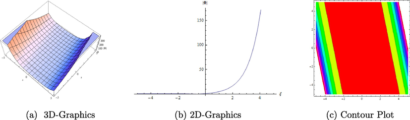
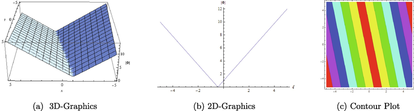
3D-graphics, 2D-graphics and contour plots of different solutions
of Eq. (1) with
are presented to describe their behaviour in Fig. 1–6.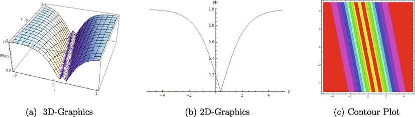
Different graphical representations of
with
.
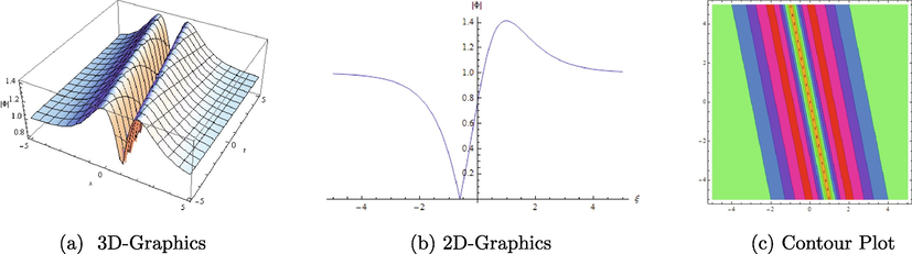
Different graphical representations of
with
.
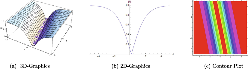
Different graphical representations of
with
.
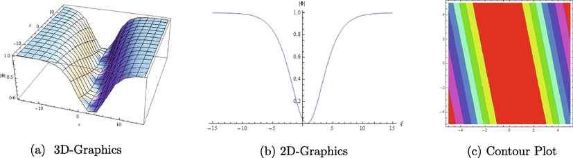
Different graphical representations of
with
.
Different graphical representations of
with
.
Different graphical representations of
with
.
3 Bifurcations behavior and phase portraits
According to ideology of the planar dynamical systems, equilibrium point is exclaimed as the saddle point if , if , then center and , a node if and while, when then zero point and Poincaré index of is zero. Where, J and exhibits the trace of coefficients matrix and also Jacobian matrix for any linearized system of (47). For the categorization of non-identical orbits in phase portraits of dynamical system (47), some symbols will be practised:
-
(1):
Super non-linear periodic orbit is manifested by SNPO(e,s),
-
(2):
Non-linear homoclinic orbit is manifested by NHO(e,s),
-
(3):
Non-linear heteroclinic orbit is manifested by NHTO(e,s),
-
(4):
Non-linear periodic orbit is manifested by NPO(e,s),
The system (47) delineates the planar Hamiltonian kind. Hamiltonian functions prevailed by integrating (47):
From (48), validity can be attested as:
As a system (47) is a planar Hamiltonian system and from (49), it can be concluded that system (47) is conservative and thus phase orbits expressed by the vector field of (47) will posses each traveling waves solution of Eq. (44) (for detail see Li et al., 2015 and references therein).
Level curves
in respect of energy level h can be defined in the following fashion:
where,
is expounded in (48) and h is known as the energy level. In phase portraits against every energy level, h one can have an orbit. To investigate the relations between closed orbit and the energy level of the system (47), let us define:
From (48), one can easily find the following relation:
System (47) has three equilibrium points:
The linearized system (47) reported as coefficient matrix at an equilibrium point
:
It yields the following cases:
3.0.1 or
There are three equilibrium points of system (47)
, and
for this type. For this
while
and
. Above information helps to claim that
is the saddle point and
are the center points (see Fig. 7(a)).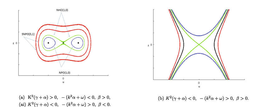
Phase portraits of nonlinear dynamical system.
For this case, the phase portraits of the nonlinear dynamical system (47) is presented in Fig. 7(a). This phase portrait encompasses a class of SNPO(3,1), where the family of SNPO(3,1) carries all included equilibrium points of the considered dynamical model. It also carries two families of NPO(1,0), which accommodates and . There is also a pair of NHO(1,0) at which carries and .
3.0.2
A single equilibrium point incorporated in the system (47), where thus is a saddle point. (see Fig. 7(b)).
3.0.3 . or
There are three equilibrium points of system (47)
, and
for this type. For this
and
, so
is the center point, while
and
with Poincarè index is zero thus
are cusp points, (see Fig. 8(a)). The phase portraits of the carried system of non-linear ODEs (47) is given in Fig. 8(a). This phase portrait carries a family of NPO(1,0) which envelops
.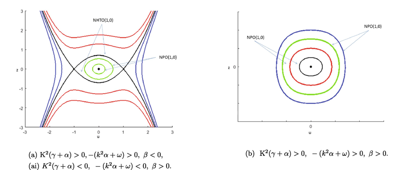
Phase portraits of nonlinear dynamical system.
3.0.4
Only single equilibrium point is assimilated in (47). For which and , thus is a center point. The phase portraits for this case is presented in Fig. 8(b), which shows that there is a family of NPO(1,0) which carries .
4 Conserved quantities
In this section, nontrivial conserved quantities (Nother et al. (1918) and Olver (1986)) are enumerated by using the method given by Anco and Bluman Anco and Bluman, 2002. They advocated a systematic approach to built non-trivial conservation laws.
Phase portraits of nonlinear dynamical system with different energy levels.
4.1 Multiplier approach
A system containing two partial differential equations of second order with three independent
and two dependent variables
and is denoted by
If
is the solution of Eq. (54), form Eq. (55), one can derive the local conserved quantity by using the following equation
System (54) contains the set of multipliers for the conserved quantities if and only if following identity holds:
Eq. (58) leads to a set of over-diagnosed system of determining equations in expressions of multipliers . The solution of the obtained determining equations with some computation further gives the conserved quantities. In this section, first-order nontrivial conserved quantities are computed by using the method given by Anco and Bluman Anco and Bluman, 2002. They advocated a systematic approach to built non-trivial conservation laws. In this method, multipliers of precise order for undertook problem is required, additionally, which is used to get their analogous fluxes . Each class of multipliers and fluxes fabricates a local conservation law holding for all solutions of considered differential equations.
4.2 Conserved quantities
In this section, conserved quantities of Eq. (1) are computed (Anco and Bluman, 2002; Cheviakov, 2007).
Eq. (44) with complex envelope:
Substituting system (61) in Eq. (58) gives:
Equating the coefficients of derivatives of dependent variables concerning independent variables in Eq. (62), we get a linear homogeneous over-determined system of partial differential equations. After solving the obtained system of partial differential equations for
with the assistance of Maple, we will secure the following consequences:
The next step is to find the fluxes by using the multiplier given in (63). For instance, the multipliers and for the constants give the following conservation laws:
-
(64)
-
(65)
-
(66)
-
(67)
4.3 Conclusion
To be brief, the new direct extended algebraic method (Rezazadeh, 2018) is applied to perceive the exact solutions of the resonant non-linear Schrödinger equation with Kerr law nonlinearity. The proffered technique gave a class of solutions that may be worthwhile for explaining certain physical phenomena accurately. Moreover, the physical composition of these solutions is described via their graphical presentation. Four portraits of a dynamical system (47) are obtained and the existence of the traveling wave solutions is discussed as well. It is observed that obtained solutions are new and not available in the literature. Further, all possible cases of the system parameters are considered by using the phase portraits, and the effect of different situations are shown in detail. Moreover, nontrivial, first order and new conserved quantities are given by using the multiplier approach.
In the future, the perturbed dynamical structure of the considered model can be investigated in light of chaos and sensitivity analysis.
5 Ethical standards
The authors state that this research complies with ethical standards. This research does not involve either human participants or animals.
Declaration of Competing Interest
The authors declare that they have no known competing financial interests or personal relationships that could have appeared to influence the work reported in this paper.
References
- Exact solutions, conservation laws, bifurcation of nonlinear and super nonlinear traveling waves for Sharma-Tasso-Olver equation. Nonlinear Dyn.. 2018;94:1791-1801.
- [Google Scholar]
- Direct construction method for conservation laws of partial differential equations Part II: General treatment. Eur. J. Appl. math.. 2002;41:567-585.
- [Google Scholar]
- Dark optical solitons and conservation laws to the resonance nonlinear Schrödingers equation with Kerr law nonlinearity. Optik. 2017;147:248-255.
- [Google Scholar]
- New Complex Hyperbolic Structures to the Lonngren-Wave Equation by Using Sine-Gordon Expansion Method. Appl. Math. Nonlinear Sci.. 2019;4(1):141-150.
- [Google Scholar]
- Introduction to Non-Kerr Law Optical Solitons. Boca Raton, FL, USA: CRC Press; 2006.
- Cattani, C., scalia, M., Laserra, E., Bochicchio, I., Nandi, K.K., 2013. Correct light deflection in Weyl conformal gravity. Phys. Rev. D 87 (4), 047503.
- GeM software package for computation of symmetries and conservation laws of differential equations. Comput. Phys. Commun.. 2007;176:48-61.
- [Google Scholar]
- Dubinov, A.E., Kolotkov, D. Yu, Sazonkin, M.A., 2012. Supernonlinear waves in plasma. Plasma Phys. Rept., 38 (10), 833–844.
- New Complex and Hyperbolic Forms for Ablowitz-Kaup-Newell-Segur Wave Equation with Fourth Order. Appl. Math. Nonlinear Sci.. 2019;4(1):105-112.
- [Google Scholar]
- Soliton solutions of the resonant nonlinear Schrödingers equation in optical fibers with time dependent coefficients by simplest equation approach. J. Mod. Opt.. 2013;60(19):1627-1636.
- [Google Scholar]
- An efficient computational method for solving nonlinear stochastic It integral equations: application for stochastic problems in physics. J. Comput. Phys.. 2015;283:148-168.
- [Google Scholar]
- Noether-type symmetries and conservation laws via partial Lagrangian. Nonlinear Dyn.. 2006;45:367-383.
- [Google Scholar]
- On optimal system, exact solutions and conservation laws of the modified equal-width equation. Appl. Math. Nonlinear Sci.. 2018;3(2):409-418.
- [Google Scholar]
- Travelling waves and conservation laws of a (2+1)-dimensional coupling system with Korteweg-de Vries equation. Appl. Math. Nonlinear Sci.. 2018;3(1):241-254.
- [Google Scholar]
- Effect of Hall current on the magneto hydrodynamic free convective flow between vertical walls with induced magnetic field. Eur. Phys. J. Plus. 2018;133:207.
- [Google Scholar]
- Influence of heat source/sink on MHD flow between vertical alternate conducting walls with Hall effect. Physica A. 2020;544 123562
- [Google Scholar]
- Bifurcation analysis and solutions of a higher order nonlinear Schrödinger’s equation. Math. Prob. Eng.. 2015;2015 408586-408585
- [Google Scholar]
- Solutions and conservation laws of a generalized second extended (3+1)-dimensional Jimbo-Miwa equation. Appl. Math. Nonlinear Sci.. 2018;3(2):459-474.
- [Google Scholar]
- Nother, E., 1918. Invariante Variationsprobleme, Nacr. König. Gesell. Wissen., Göttingen, Math.-phys. Kl. Heft, 2, 235–257 (English translation in Transport Theory and Statistical Physics, 1(3), (1971) 186–207.
- Applications of Lie Groups to Differential Equations. New York: Springer-Verlag; 1986.
- New soliton solutions of the complex Ginzburg-Landau equation with Kerr law nonlinearity. Optik. 2018;167:218-227.
- [Google Scholar]
- Wavelet analysis of the evolution of a solitary wave in a composite material. Int. Appl. Mech.. 2004;40:311-318.
- [Google Scholar]
- Numerical simulation for fractional-order Bloch equation arising in nuclear magnetic resonance by using the Jacobi polynomials. Appl. Sci.. 2020;10(8):2850.
- [Google Scholar]
- Singh, H. Numerical simulation for fractional delay differential equations. Int. J. Dyn. Control doi: 10.1007/s40435-020-00671-6.
- Analysis for fractional dynamics of Ebola virus models. Chaos Solitons Fract.. 2020;138 109992
- [Google Scholar]
- Solving Non-Linear Fractional Variational Problems Using Jacobi Polynomials. Mathematics. 2019;7(3):224.
- [Google Scholar]
- Legendre spectral method for the fractional Bratu problem. Math. Meth. Appl. Sci.. 2020;43(9):5941-5952.
- [Google Scholar]
- Magnetohydrodynamic flow in horizontal concentric cylinders. Inter. J. Indus. Math.. 2019;11:89-98.
- [Google Scholar]
- Bifurcation analysis and the travelling wave solutions of the Klein-Gordon-Zakharov equations. Pramana J. Phys.. 2013;80(1):41-59.
- [Google Scholar]


