Modified Double Conformable Laplace Transform and Singular Fractional Pseudo-Hyperbolic and Pseudo-Parabolic Equations

1 Introduction

Subject area of (DCLTs) and its attributes are still fresh, some properties and definitions of fractional calculus were also considered in Abdeljawad (2015), Alderremy et al. (2018), Atangana et al. (2015), and Baleanu et al. (2019), Some fractional partial differential equations were also solved (Gadain, 2017; Khalil et al., 2014), many researchers have given their attention to examining the solutions of fractional linear and nonlinear PDEs by different methods (Mustafa Inc et al., 2018, 2019; Aliyu, et al., 2019). Along with these attacks are the Elzaki transform (Elzaki, 2014; Elzaki and Eman, 2012; Elzaki and Alderremy, 2018), Homotopy perturbation method (Mohamed and Elzaki, 2020), Laplace transforms (Korkmaz, 2018), and double Laplace transform (Elzaki 2012) (Fig. 1).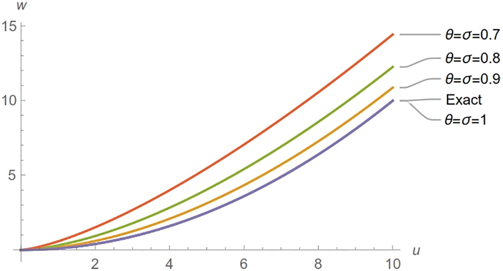

Close

Fig. 1

Exact and approximate solutions for Example1.

Export to PPT

In this theme, we will inaugurate a novel double conformable Laplace's transform and a few of its attributes and mix this transform with the new method to figure out the singular fractional Pseudo-hyperbolic and Pseudo-parabolic equations. The robustness and the effectiveness of the proposed method lies in the fact that it found the exact solution by taking only one approximation, while the other methods take a several of approximations (Fig. 2).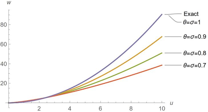

Close

Fig. 2

Exact and approximate solutions for Example 2.

Export to PPT

We think that the double conformable Laplace's transform technique is expanded in the near future to solve a real model problem that related to Fractional Pseudo-hyperbolic or Pseudo-parabolic equations in science and engineering such heat and mass transfer problem (Emmanuel et al., 2018), fluid flow problem, quantum mechanics, (Aliyu et al., 2019) etc.

1. the conformable single Laplace transform (CSLT) with respect to $u,$ designated by the operator ${\ell }_u^{\theta }\left[\mathrm{\Omega }(u,w)\right]$ , is defined by:

(ii) the (CSLT) with respect to $w,$ of $\mathrm{\Omega }(u,w)$ , is,

(iii) The conformable double Laplace’s transform (CDLT) of, is,

Note that: ${\ell }_w^{\sigma }{\ell }_u^{\theta }\left[\mathrm{\Omega }(u,w)\right]={\ell }_u^{\theta }{\ell }_w^{\sigma }\left[\mathrm{\Omega }(u,w)\right]=\mathrm{\Phi }(r,v)$

Also, we see the (CDLT) of the following functions, $${\ell }_w^{\sigma }{\ell }_u^{\theta }\left[e^{\frac{w^{\sigma }}{\sigma }+\frac{u^{\theta }}{\theta }}\right]=\frac{1}{(v-1)(r-1)},{\ell }_w^{\sigma }{\ell }_u^{\theta }\left[cos\frac{u^{\theta }}{\theta }\right]=\frac{r}{v(r^2+1)},{\ell }_w^{\sigma }{\ell }_u^{\theta }\left[sin\frac{u^{\theta }}{\theta }\right]=\frac{1}{v(r^2+1)}$$

For proof and more details, see [3,13].

2 Method of solution

To explicate the method of solution, we will think about the following fractional PDE,

With the initial conditions,

$\eta =1,$ for a fractional Pseudo-parabolic equation, and $\eta =2,$ for a fractional Pseudo-hyperbolic equation, In this general study, we put $\eta =2,$ $w{D}_{\sigma }^{\eta }\mathrm{\Omega }(u,w),$ is the $\sigma$ ^th, order conformable fractional partial derivative of $\mathrm{\Omega }(u,w)$ . $R$ and, $N$ are a linear operator and a nonlinear operator respectively.

To, obtain the result of the Eqs. (6), (7), we get hold of the (CDLT) of Eq.(6), and (CSLT) of Eq. (7), to obtain,

And,

Let:

is the a solution of Eq. (6).

After substituting Eq. (9), in Eq. (8), taking the conformable inverse of (DLT) of Eq. (8), to obtain, $$\mathrm{\Omega }(u,w)=F\left(\frac{u^{\theta }}{\theta },\frac{w^{\sigma }}{\sigma }\right)+{\left({\ell }_w^{\sigma }\right)}^{-1}{\left({\ell }_u^{\theta }\right)}^{-1}\left\{\frac{1}{v^2}{\ell }_w^{\sigma }{\ell }_u^{\theta }\left[f(u,w)-R\mathrm{\Omega }(u,w)-N\mathrm{\Omega }(u,w)\right]\right\}$$

In lodge to obtain the exact solution by selecting only one measure, we must prefer the best initial iteration ${\mathrm{\Omega }}_0(u,w),$

if we choose, ${\mathrm{\Omega }}_0(u,w)=F\left(\frac{u^{\theta }}{\theta },\frac{w^{\sigma }}{\sigma }\right)$ then, the recursive relation is,

And then we can find the solution by using Eqs. (10), (11).

3 Application

To demonstrate the productivity of this technique in solves the singular fractional Pseudo-hyperbolic and singular fractional Pseudo-parabolic equations, by accepting just one step, we establish the previous examples.

with,

Practicing the same steps mentioned as before to obtain,

By definition 1.4 and the initial condition (13), Eq. (14) becomes,

Getting hold of the conformable inverse of (DLT) of Eq. (15), to obtain, $\mathrm{\Omega }(u,w)={\left(\frac{x^{\theta }}{\theta }\right)}^{2}sin\frac{t^{\sigma }}{\sigma }+{\left({\ell }_w^{\sigma }\right)}^{-1}{\left({\ell }_u^{\theta }\right)}^{-1}\left\{\frac{1}{v}{\ell }_w^{\sigma }{\ell }_u^{\theta }\left[\begin{array}{c}\frac{1}{u}u{D}_{\theta }\left(u\left(u{D}_{\theta }\mathrm{\Omega }(u,w)\right)\right)+\frac{1}{x}wu{D}_{\sigma \theta }^2\left(u\left(u{D}_{\theta }\mathrm{\Omega }(u,w)\right)\right)\\ -4sin\frac{w^{\sigma }}{\sigma }-4cos\frac{w^{\sigma }}{\sigma }\end{array}\right]\right\}$

Then the recursive relation is,

The first few components are given by, $${\mathrm{\Omega }}_0(u,w)={\left(\frac{u^{\theta }}{\theta }\right)}^{2}sin\frac{w^{\sigma }}{\sigma },{\mathrm{\Omega }}_1(u,w)={\left({\ell }_w^{\sigma }\right)}^{-1}{\left({\ell }_u^{\theta }\right)}^{-1}\left\{\frac{1}{v}{\ell }_w^{\sigma }{\ell }_u^{\theta }\left[0\right]\right\}=0,...$$

If we use Eq. (10), then the solution of the Eq. (12) is, $$\mathrm{\Omega }(u,w)={\left(\frac{u^{\theta }}{\theta }\right)}^{2}sin\frac{w^{\sigma }}{\sigma },$$

We can see if $\theta =\sigma =1,$ then the exact solution is, $\mathrm{\Omega }(u,w)=u^{2}sinw$ , is bounded.

With,

Using the same steps which we used in example 1, to prevail; $$\mathrm{\Phi }(r,v)=\frac{1}{v^2}\left[\frac{2}{r^3\left(v^2+1\right)}+\frac{2v}{r^3}-\frac{2}{r^3}\right]+\frac{1}{v^2}{\ell }_w^{\sigma }{\ell }_u^{\theta }\left[\begin{array}{c}\frac{1}{u}u{D}_{\theta }\left(u\left(u{D}_{\theta }\mathrm{\Omega }(u,w)\right)\right)+\frac{1}{u}wu{D}_{\sigma \theta }^2\left(u\left(u{D}_{\theta }\mathrm{\Omega }(u,w)\right)\right)\\ +\frac{1}{2}\left(\frac{u^{\theta }}{\theta }\right)\mathrm{\Omega }(u,w)\left(u{D}_{\theta }\mathrm{\Omega }(u,w)\right)-{\mathrm{\Omega }}^2(u,w)\end{array}\right]$$

Getting hold of the conformable inverse of (DLT) of the last equation to make, $$\mathrm{\Omega }(u,w)={\left(\frac{u^{\theta }}{\theta }\right)}^2{e}^{-\frac{w^{\sigma }}{\sigma }}+{\left({\ell }_w^{\sigma }\right)}^{-1}{\left({\ell }_u^{\theta }\right)}^{-1}\left\{\frac{1}{v^2}{\ell }_w^{\sigma }{\ell }_u^{\theta }\left[\begin{array}{c}\frac{1}{u}u{D}_{\theta }\left(u\left(u{D}_{\theta }\mathrm{\Omega }(u,w)\right)\right)+\frac{1}{u}wu{D}_{\sigma \theta }^2\left(u\left(u{D}_{\theta }\mathrm{\Omega }(u,w)\right)\right)\\ +\frac{1}{2}\left(\frac{u^{\theta }}{\theta }\right)\mathrm{\Omega }(u,w)\left(u{D}_{\theta }\mathrm{\Omega }(u,w)\right)-{\mathrm{\Omega }}^2(u,w)\end{array}\right]\right\}$$

Thus, we be able to write down the recursive relations as, $$\begin{array}{c}{\mathrm{\Omega }}_{n+1}(u,w)={\left({\ell }_w^{\sigma }\right)}^{-1}{\left({\ell }_u^{\theta }\right)}^{-1}\left\{\frac{1}{v^2}{\ell }_w^{\sigma }{\ell }_u^{\theta }\left[\begin{array}{c}\frac{1}{u}u{D}_{\theta }\left(u\left(u{D}_{\theta }{\mathrm{\Omega }}_n(u,w)\right)\right)-{\mathrm{\Omega }}_n^2(u,w)\\ +\frac{1}{u}wu{D}_{\sigma \theta }^2\left(u\left(u{D}_{\theta }{\mathrm{\Omega }}_n(u,w)\right)\right)+\frac{1}{2}\left(\frac{u^{\theta }}{\theta }\right){\mathrm{\Omega }}_n(u,w)\left(u{D}_{\theta }{\mathrm{\Omega }}_n(u,w)\right)\end{array}\right]\right\}\\ {\mathrm{\Omega }}_0(u,w)={\left(\frac{u^{\theta }}{\theta }\right)}^2{e}^{-\frac{w^{\sigma }}{\sigma }}\end{array}$$

And so the first few components are, $${\mathrm{\Omega }}_0(u,w)={\left(\frac{u^{\theta }}{\theta }\right)}^2{e}^{-\frac{w^{\sigma }}{\sigma }},{\mathrm{\Omega }}_1(u,w)={\left({\ell }_w^{\sigma }\right)}^{-1}{\left({\ell }_u^{\theta }\right)}^{-1}\left\{\frac{1}{v^2}{\ell }_w^{\sigma }{\ell }_u^{\theta }\left[0\right]\right\},...$$

Then, the solution of Eq. (17) is, $$\mathrm{\Omega }(u,w)={\left(\frac{u^{\theta }}{\theta }\right)}^2{e}^{-\frac{w^{\sigma }}{\sigma }},$$

If $\theta =\sigma =1,$ then, the exact solution is, $\mathrm{\Omega }(u,w)=u^2{e}^{-w}.$ is bounded.

4 Conclusion

The (CDLT) and a few of its properties were studied, also we study the (CDLT) of fractional derivatives and few functions, and then we combine (CDLT) with a new method to solve a new type of fractional partial differential equations called “Singular Fractional Pseudo-hyperbolic and Pseudo-parabolic Equations”. This method is extremely easy and useful to solve these fractional differential equations which are related with the engineering and physical sciences because we get the exact solution by taking just one step compared with other methods that require several steps to get the exact solution.

We will look at possibility of tackle fractional Pseudo- elliptic Equations using this method in the future study.

References

- Dynamics of optical solitons, multipliers and conservation laws to the nonlinear schrödinger equation in (2+1)-dimensions with non-Kerr law nonlinearity. J. Mod. Opt.. 2019;66(2):136-142.
- [CrossRef] [Google Scholar]
- New transform iterative method for solving some Klein-Gordon equations. Results Phys.. 2018;10:655-659.
- Dumitru Baleanu, Mustafa Inc, Aliyu Isa Aliyu & Abdullahi Yusuf (2019) The investigation of soliton solutions and conservation laws to the coupled generalized Schrödinger–Boussinesq system, Waves in Random and Complex Media, 29:1, 77- .92, DOI: 10.1080/17455030.2017.1412539.
- Jesús Emmanuel, Solís Pérez, José Francisco Gómez-Aguilar, Dumitru Baleanuand Fairouz Tchier, 2018. Chaotic attractors with fractional conformable derivatives in the Liouville-Caputo sense and its dynamical behaviors. Entropy, 20 (5), 384.
- Application of double Laplace decomposition method for solving singular one dimensional system of hyperbolic equations. J. Nonlinear Sci. Appl.. 2017;10:111-121.
- [Google Scholar]
- On the wave solutions of conformable fractional evolution equations. Commun. Fac. Sci. Univ. Ank. Ser. A1. 2018;67(1):68-79.
- Mohamed Z. Mohamed, Tarig M. Elzaki, 2020. Applications of new integral transform for linear and nonlinear fractional partial differential equations, Journal of King Saud University – Science, 32, 544–549. https://doi.org/10.1016/j.jksus.2018.08.003.
- Mustafa Inc , Hamdy I. Abdel Gawad, Mohammad Tantawy, Abdullahi Yusuf, 2019. On multiple soliton similariton‐pair solutions, conservation laws via multiplier and stability analysis for the Whitham–Broer–Kaup equations in weakly dispersive media, Mathem. Methods Appl. Sci., 42(7), (2019) 2455–2464.
- Mustafa Inc, Aliyu Isa Aliyu, Abdullahi Yusuf, Dumitru Baleanu, (2018), Novel optical solitary waves and modulation instability analysis for the coupled nonlinear Schrödinger equation in monomode step-index optical fibers, Superlatt. Microstruct. 113 (2018) 745–753.
- On the new double integral transform for solving singular system of hyperbolic equations. J. Nonlinear Sci. Appl.. 2018;11:1207-1214. Available online at www.isr-publications.com/jnsa
- Application of projected differential transform method on nonlinear partial differential equations with proportional delay in one variable. World Appl. Sci. J.. 2014;30(3):345-349.
- Tarig M. Elzaki, 2012. Double laplace variational iteration method for solution of nonlinear convolution partial differential equations, Archives Des Sciences, ISSN 1661-464X, Vol. 65, No. 12, PP. 588–593.
- Tarig M. Elzaki, Eman M.A. Hilal, 2012. Solution of Telegraph Equation by Modified of Double Sumudu Transform “Elzaki Transform” , Mathematical Theory and Modeling, ISSN 2224-5804 (Paper) ISSN 2225-0522 (Online), Vol.2, No.4, pp, 95-103.