Modeling engineering data using extended power-Lindley distribution: Properties and estimation methods

Abdulhakim A. Al-Babtain; Devendra Kumar; Ahmed M. Gemeay; Sanku Dey; Ahmed Z. Afify

doi:10.1016/j.jksus.2021.101582

View/Download PDF

Buy Reprints

PDF

Translate this page into:

12 2021

:33;

101582

doi:

10.1016/j.jksus.2021.101582

Modeling engineering data using extended power-Lindley distribution: Properties and estimation methods

Abdulhakim A. Al-Babtain^{^a}, Devendra Kumar^{^b,⁎}, Ahmed M. Gemeay^{^c}, Sanku Dey^{^d}, Ahmed Z. Afify^{^e}

a Department of Statistics and Operations Research, King Saud University, Riyadh 11362, Saudi Arabia

b Department of Statistics, Central University of Haryana, India

c Department of Mathematics, Faculty of Science, Tanta University, Tanta 31527, Egypt

d Department of Statistics, St. Anthony’s College, Shillong, Meghalaya 793001, India

e Department of Statistics, Mathematics and Insurance, Benha University, Benha 13511, Egypt

⁎Corresponding author at: Department of Statistics, Central University of Haryana, India. devendrastats@gmail.com (Devendra Kumar)

Received: 2021-1-8, Accepted: 2021-8-19,

Disclaimer:
This article was originally published by Elsevier and was migrated to Scientific Scholar after the change of Publisher.

Peer review under responsibility of King Saud University.

Abstract

In this paper, we introduce a new flexible distribution called the Weibull Marshall-Olkin power-Lindley (WMOPL) distribution to extend and increase the flexibility of the power-Lindley distribution to model engineering related data. The WMOPL has the ability to model lifetime data with decreasing, increasing, J-shaped, reversed-J shaped, unimodal, bathtub, and modified bathtub shaped hazard rates. Various properties of the WMOPL distribution are derived. Seven frequentist estimation methods are considered to estimate the WMOPL parameters. To evaluate the performance of the proposed methods and provide a guideline for engineers and practitioners to choose the best estimation method, a detailed simulation study is carried out. The performance of the estimators have been ranked based on partial and overall ranks. The performance and flexibility of the introduced distribution are studied using one real data set from the field of engineering. The data show that the WMOPL model performs better than some well-known extensions of the power-Lindley and Lindley distributions.

Keywords

Anderson–Darling estimation

Maximum likelihood estimation

Maximum product of spacing

Moments

Power-Lindley distribution

Show Related Articles from PubMed

1 Introduction

The life length of any system and/or device can be usually described by means of lifetime distributions. The most commonly used lifetime distributions are the exponential, Weibull, Lindley, and gamma distributions. However, many real lifetime data can not be modeled effectively using classical distributions. Owing to this, there is a growing interest in statistical literature to develop more flexible distributions in the distribution theory which capable of modeling several real data in applied areas such as engineering and reliability. Among the new generalized models, the generalizations of the Lindley distribution have become popular in recent times as it is observed that in several cases, the Lindley model and its generalizations are capable of modelling lifetime data adequately. Hence, several researchers are focusing on finding new generalizations/extensions of the Lindley distribution to describe lifetime phenomena in many applied areas. Modeling real data using generalized distributions is an open problem and consequently many generalized distributions have been developed and applied in several fields. Nevertheless, there are still many important problems involving real data, which are not addressed by known models.

Lindley distribution was proposed by Lindley (Lindley, 1958) as a mixture of exponential and gamma distributions in the context of fiducial and Bayesian statistics. Ghitany et al. (Ghitany et al., 2008) studied some of its structural properties and pointed out that it is more suitable for modelling waiting times before service of bank customers data than the exponential distribution. The statistical literature abounds in many extended forms of Lindley distribution. For example, the generalized Lindley (Zakerzadeh and Dolati, 2009), negative binomial Lindley (Zamani and Ismail, 2010), generalized Poisson Lindley (Mahmoudi and Zakerzadeh, 2010), transmuted Lindley (Merovci, 2013), power-Lindley (PL) (Ghitany et al., 2013), complementary geometric transmuted-Lindley (Afify et al., 2016), Weibull Lindley (Asgharzadeh et al., 2018) and extended odd Weibull Lindley distributions (Alizadeh et al., 2018) and so on. Furthermore, Al-Babtain et al. (Al-Babtain et al., 2020) introduced the natural discrete Lindely as a mixture of negative binomial and geometric distributions.

For any baseline G distribution with parameter vector $φ$ , Korkmaz et al. (Korkmaz et al., 2019) proposed the Weibull Marshall-Olkin-G (WMO-G) family based on the T-X generator introduced by Alzaatreh et al. (Alzaatreh et al., 2013). The cumulative distribution function (CDF) of the T-X generator is defined by

(1)

F (x) = \int_{a}^{W [G (x; φ)]} r (t) dt = R (W [G (x; φ)]) .

Setting $r (t) = β t^{θ - 1} e^{- t^{θ}}, t > 0$ , with shape parameter $θ > 0$ and $W [G (x; φ)] = - \log [\frac{α \bar{G} (x; φ)}{G (x; φ) + λ \bar{G} (x; φ)}], λ > 0 .$

Hence, the CDF of the WMO-G family takes the form

(2)

F (x; λ, θ, φ) = 1 - \exp (- {\{- \log [\frac{λ \bar{G} (x; φ)}{1 - \bar{λ} \bar{G} (x; φ)}]\}}^{θ}) .

The corresponding probability density function (PDF) of (2) is defined as

(3)

\begin{matrix} f (x; λ, θ, φ) = & \frac{θ g (x; φ)}{\bar{G} (x; φ) [1 - \bar{λ} \bar{G} (x; φ)]} {\{- \log [\frac{λ \bar{G} (x; φ)}{1 - \bar{λ} \bar{G} (x; φ)}]\}}^{θ - 1} \\ \times & \exp (- {\{- \log [\frac{λ \bar{G} (x; φ)}{1 - \bar{λ} \bar{G} (x; φ)}]\}}^{θ}), \end{matrix}

where

g (x; φ)

is the baseline PDF,

\bar{λ} = 1 - λ

, and

λ

and

θ

are two extra positive shape parameters.

The hazard rate function (HRF) of the WMO-G family is $h (x; λ, θ, φ) = \frac{θ W (x, φ)}{[1 - \bar{λ} \bar{G} (x; φ)]} {\{- \log [\frac{λ \bar{G} (x; φ)}{1 - \bar{λ} \bar{G} (x; φ)}]\}}^{θ - 1},$ where $W (x; φ) = g (x; φ) / [1 - G (x; φ)]$ is the HRF of the baseline model.

The Weibull-X family (Alzaatreh et al. (Alzaatreh et al., 2013), Cordeiro et al. (Cordeiro et al., 2015)) follows as special case from the WMO-G family with $λ = 1$ . The MO-G family (Marshall and Olkin (Marshall and Olkin, 1997)) is obtained as a special class from the WMO-G family with $θ = 1$ . The baseline distribution follows from the WMO-G family for $λ = θ = 1$ . More details on the WMO-G family can be explored in Korkmaz (Korkmaz et al., 2019).

Motivated by this rationale, we introduce a new four-parameter lifetime distribution called the Weibull Marshall-Olkin power-Lindley (WMOPL) distribution as a generalization of two parameter PL distribution and to study some of its properties. The WMOPL distributions generalizes the PL model (Ghitany et al., 2013), Marshall-Olkin PL (MOPL) (Hibatullah et al., 2018), WMO-Lindley (WMOL) (Afify et al., 2020b) distributions among others. The importance of the new distribution is the ability of describing real data-set with decreasing, increasing, J-shaped, reversed-J shaped, unimodal, bathtub, and modified bathtub shaped hazard rate functions better than at least eighteen well known lifetime extensions of the Lindley and power-Lindley distributions as we show later. Its density function admits a linear mixture representation of PL densities. Next, we estimate the WMOPL parameters using different classical methods of estimation and determine the best estimation method for the WMOPL parameters which may be of great help to applied statisticians and engineers. The considered estimators include the maximum likelihood estimators (MLEs), least squares estimators (LSEs), maximum product of spacings estimators (MPSEs), weighted least squares estimators (WLSEs), Cramer-von-Mises estimators (CMEs), Anderson–Darling estimators (ADEs) and right-tail Anderson–Darling estimators (RADEs). To evaluate the performance of the proposed estimators, we conduct a detailed simulation study for medium and large sample sizes.

A random variable (rv) X is said to follow the PL distribution if its PDF and CDF are given by $g (x) = \frac{τ δ^{2}}{1 + δ} (1 + x^{τ}) x^{τ - 1} e^{- δ x^{τ}}, x > 0, δ, τ > 0$ and $G (x) = 1 - (\frac{1 + δ + δ x^{τ}}{1 + δ}) e^{- δ x^{τ}}, x > 0, δ, τ > 0 .$

To this end, the CDF of the WMOPL distribution follows, by setting the CDF of the PL model in (2), as

(4)

F (x; λ, θ, δ, τ) = 1 - \exp \{- {[\log (\frac{(1 + δ) e^{δ x^{τ}}}{λ (1 + δ + δ x^{τ})} - \frac{\bar{λ}}{λ})]}^{θ}\} .

The WMOPL PDF corresponding to (4) takes the form

(5)

\begin{matrix} f (x; λ, θ, δ, τ) = & \frac{θ τ δ^{2} x^{τ - 1} (1 + x^{τ}) {(1 + δ + δ x^{τ})}^{- 1}}{1 - (\frac{1 + δ + δ x^{τ}}{1 + δ}) \bar{λ} e^{- δ x^{τ}}} \times {\{\log [\frac{(1 + δ) e^{δ x^{τ}}}{λ (1 + δ + δ x^{τ})} - \frac{\bar{λ}}{λ}]\}}^{θ - 1} \\ \times & \exp \{- {[\log (\frac{(1 + δ) e^{δ x^{τ}}}{λ (1 + δ + δ x^{τ})} - \frac{\bar{λ}}{λ})]}^{θ}\}, \end{matrix}

where

\bar{λ} = 1 - λ, λ > 0, θ > 0

and

τ > 0

are two shape parameters and

δ > 0

is a scale parameter.

Henceforth, $X \sim WMOPL (λ, θ, δ, τ)$ denotes arv with PDF (5).

The HRF of the WMOPL model takes the form $h (x; λ, θ, δ, τ) = \frac{θ τ δ^{2} x^{τ - 1} (1 + x^{τ})}{(1 + δ + δ x^{τ}) [1 - (\frac{1 + δ + δ x^{τ}}{1 + δ}) \bar{λ} e^{- δ x^{τ}}]} {\{\log [\frac{(1 + δ) e^{δ x^{τ}}}{λ (1 + δ + δ x^{τ})} - \frac{\bar{λ}}{λ}]\}}^{θ - 1} .$

The WMOPL distribution contains some special cases such as the Weibull-PL distribution (for $λ = 1$ ), the MOPL distribution (for $θ = 1$ ), the WMOL distribution (for $τ = 1$ ), and the PL distribution (for $λ = θ = 1$ ).

Some possible shapes for the PDF and HRF of the WMOPL distribution are depicted graphically in Figs. 1 and 2, respectively.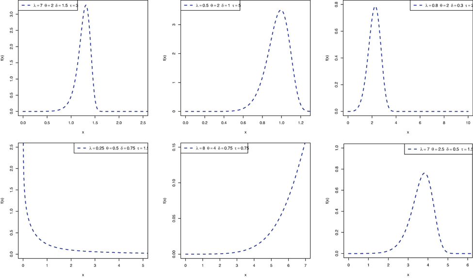

Plots of WMOPL PDF for different parametric values.

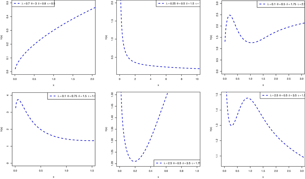
Plots of WMOPL HF for different parametric values.

The article is organized as follows. In the next section, we provide some properties of the WMOPL distribution. In Section 3, different frequentist methods of estimation are discussed. Monte Carlo simulation study is carried out to compare the different methods of estimation in Section 4. The potentiality of the WMOPL model is illustrated by means of one engineering related data set in Section 5. Finally, some concluding remarks are addressed in Section 6.

2 Properties of the WMOPL distribution

Some mathematical properties of the WMOPL distribution are presented in this section. We consider only the case $0 < λ < 1$ , since for $λ > 1$ all equations derived hold by changing the coefficients $w_{k, l}$ by $ν_{k, l}$ .

2.1

2.1 Linear representation

To have a linear representation for the WMOPL PDF based on power series $e^{x} = \sum_{i = 0}^{\infty} \frac{x^{i}}{i!},$ the exponential part of the CDF of X can be expressed from (4) as

(6)

F (x) = \sum_{i = 1}^{\infty} \frac{{(- 1)}^{i + 1}}{i!} {[- \log \{1 - (1 - \frac{λ (\frac{1 + δ + δ x^{τ}}{1 + δ}) e^{- δ x^{τ}}}{1 - \bar{λ} (\frac{1 + δ + δ x^{τ}}{1 + δ}) e^{- δ x^{τ}}})\}]}^{i θ} .

For $z \in (0, 1)$ and any real parameter b, the formula holds

(7)

{[- \log (1 - z)]}^{b} = z^{b} + \sum_{j = 0}^{\infty} ϕ_{j} (b) z^{j + b + 1},

where

\begin{matrix} ϕ_{0} = & \frac{1}{2} b, \\ ϕ_{1} = & \frac{1}{24} [b (3 b + 5)], \\ ϕ_{2} = & [b (b^{2} + 5 b + 6)], \\ ϕ_{3} = & \frac{1}{5760} [b (15 b^{3} + 150 b^{2} + 485 b + 502)], \dots \end{matrix}

are Stirling polynomials. The previous results were used by Cordeiro et al. (Cordeiro et al., 2015). We can write

(8)

{[- \log (1 - x)]}^{i θ} = \sum_{j = 0}^{\infty} ϕ_{j - 1} (i θ) x^{j + i θ},

where

ϕ_{j - 1} (i θ) = 0

by convention and

ϕ_{j - 1} (i θ)

(for

j ⩾ 0

) follows from (7). Then, the CDF (6) can be expressed by (8) as

F (x) = \sum_{i = 1}^{\infty} \frac{{(- 1)}^{i + 1}}{i!} ϕ_{j - 1} (i θ) {[1 - \frac{λ (\frac{1 + δ + δ x^{τ}}{1 + δ}) e^{- δ x^{τ}}}{1 - \bar{λ} (\frac{1 + δ + δ x^{τ}}{1 + δ}) e^{- δ x^{τ}}}]}^{j + i θ} .

The following power series holds for a real non-integer b and $| z | < 1$ , ${(1 - z)}^{b} = \sum_{k = 0}^{\infty} {(- 1)}^{k} (\binom{b}{k}) z^{k},$ where $(\binom{b}{k})$ = $(b (b - 1) (b - 2) (b - k + 1)) / k!$ is defined for any real b. Hence, one can obtain $\begin{matrix} F (x; λ, θ, δ, τ) = & \sum_{i = 1}^{\infty} \sum_{j, k = 0}^{\infty} \frac{{(- 1)}^{i + k + 1} λ^{k} ϕ_{j - 1} (i θ)}{i!} (\binom{i θ + k}{k}) \times {(\frac{1 + δ + δ x^{τ}}{1 + δ} e^{- δ x^{τ}})}^{k} \\ \times & {[1 - \bar{λ} (\frac{1 + δ + δ x^{τ}}{1 + δ}) e^{- δ x^{τ}}]}^{- k} . \end{matrix}$

Consider the convergent power series expression (for $| d | < 1$ and $p > 0$ ) ${(1 - d)}^{- p} = \sum_{l = 0}^{\infty} {(- 1)}^{l} (\binom{- p}{l}) d^{l} .$

For $λ \in (0, 1)$ , we can rewrite $F (x)$ as

(9)

F (x) = \sum_{k, l = 0}^{\infty} W_{k, l} {(\bar{G} (x))}^{k + l},

where

W_{k, l} = \sum_{i = 1}^{\infty} \sum_{j = 0}^{\infty} \frac{{(- 1)}^{i + k + l + 1} λ^{k} ϕ_{j - 1} (i θ)}{i! {(1 - λ)}^{- l}} (\binom{i θ + k}{k}) (\binom{- k}{l})

and

\bar{G} (x; δ) = 1 - G (x; δ)

is the PL survival function (SF).

Consider the Lehmann type II (LTII) CDF which is defined, for a baseline CDF, by $G (x)$ $Π_{c} (x) = 1 - {[1 - G (x)]}^{c}$ with power parameter (PoPa) $c > 0$ . Hence, the PDF of the LTII reduces to $π_{c} (x) = cG {(x)}^{c - 1} g (x)$ , where $g (x) = dG (x) / dx$ .

Consider the set of non-negative integers, say $J = (k, l); k, l = 0, 1, 2, \dots; k + l ⩾ 1$ .

Differentiating Eq. (9), the PDF of X follows as

(10)

f (x) = \sum_{(k, l) \in J}^{.} W_{k, l} π_{k + l} (x; λ, θ, δ, τ),

where

π_{k + l} (x) = (k + l) \bar{G} {(x; λ, θ, δ, τ)}^{k + l - 1} g (x; λ, θ, δ, τ)

denotes the PDf of the LTII-PL model with PoPa

k + l

Otherwise, if $λ > 1$ , we can write (10) as $\begin{matrix} F (x) = & \sum_{i = 1}^{\infty} \sum_{j, k = 0}^{\infty} \frac{{(- 1)}^{i + k + 1} λ^{k} ϕ_{j - 1} (i θ)}{i!} \\ \times & (\binom{i θ + k}{k}) {(\frac{1 + δ + δ x^{τ}}{1 + δ} e^{- δ x^{τ}})}^{k} \\ \times & λ^{- k} {[1 - (1 - λ^{- 1}) \frac{1 + δ + δ x^{τ}}{1 + δ} e^{- δ x^{τ}}]}^{- k} . \end{matrix}$

By using previous series expressions, we obtain

(11)

F (x) = \sum_{k, l = 0}^{\infty} ν_{k, l} π_{k + l} (x; λ, θ, δ, τ),

Eqs. (10) and (11) reveal that the PDF of the WMOPL model for the two cases are linear combination of LTII-PL densities.

Every LTII-PL can be expressed in terms of exponentiated-PL (EPL) desnities. By expanding $Π_{c} (x) = 1 - {1 - G (x)}^{c}$ (for c real), the power series converges everywhere $Π_{c} (x) = \sum_{r = 1}^{\infty} {(- 1)}^{r + 1} (\binom{c}{r}) {(G (x))}^{r} .$

By differentiating the above equation, we get

(12)

π_{c} (x) = \sum_{r = 0}^{\infty} {(- 1)}^{r} (\binom{c}{r + 1}) ρ_{r + 1} (x),

where

ρ_{r + 1} (x) = (r + 1) G {(x)}^{r} g (x)

is the EPL PDF with PoPa

r + 1

. If c is a positive integer, the last sum stops at c.

Hence, some structural properties of the WMOPL distribution can be determined from those of the EL distribution reported by Nadarajah et al. (Nadarajah et al., 2011).

2.2

2.2 Quantile function and moments

The quantile function (QF) of the WMOPL distribution takes the form

(13)

Q (p) = {\{- 1 - \frac{1}{δ} - \frac{1}{δ} W [- \frac{(δ + 1) e^{- δ - 1}}{1 - λ + λ e^{{(- 1)}^{1 / θ} \sqrt[θ]{\log (1 - p)}}}]\}}^{1 / τ}, 0 < p < 1,

We obtain the moments and moment generating function (MGF) of $X \sim$ WMOPL $(λ, θ, δ, τ)$ . Nadarajah et al. (Nadarajah et al., 2011) defined and computed $K (p, q, c, δ) = \int_{0}^{\infty} x^{c} (1 + x) {[1 - \frac{1 + q + qx}{1 + q} e^{- qx}]}^{p - 1} e^{- δ x} dx,$ which can be used to produce the rth moment $μ_{r}^{'} = E (X^{r})$ . We can write

(14)

K (p, q, c, δ) = \sum_{u = 0}^{\infty} \sum_{v = 0}^{u} \sum_{w = 0}^{v + 1} (\binom{p - 1}{u}) (\binom{u}{v}) (\binom{v + 1}{w}) \frac{{(- 1)}^{u} q^{v} Γ (w + c + 1)}{{(1 + q)}^{u} {(qu + δ)}^{w + c + 1}} .

The nth ordinary moment $μ_{n}^{'} = E (X^{n})$ can be calculated by using (9), (10) and (11). Hence $μ_{n}^{'}$ is given by $μ_{n}^{'} = \frac{δ^{2}}{{(1 + δ)}^{i + 1}} \sum_{(k, l) \in J} \sum_{r = 0}^{k + l} {(- 1)}^{r} (\binom{k + l}{r + 1}) (r + 1) W_{k, l} K ((r + 1), δ, n, δ) .$

Analogously, the MGF of X can be determined (for $t < δ$ ) as $M (t) = \frac{δ^{2}}{{(1 + δ)}^{i + 1}} \sum_{(k, l) \in J} \sum_{r = 0}^{k + l} {(- 1)}^{r} (\binom{k + l}{r + 1}) (r + 1) W_{k, l} K ((r + 1), δ, 0, δ - t) .$

3 Methods of estimation

This section is devoted to discussing seven estimation approaches of the WMOPL parameters called the MLEs, ADEs, CMEs, MPSEs, LSEs, RADEs, and WLSEs. It is worth mentioning that, several authors have been studied the estimation of the model parameters using classical estimation methods. For example, (Afify et al., 2020a; Afify and Mohamed, 2020; Al-Babtain et al., 2021; Al-Mofleh et al., 2020; Nassar et al., 2020a,b ).

3.1

3.1 Maximum likelihood estimators

The maximum likelihood estimation (MLE) is the most important method to estimate parameters of a given distribution due to its desirable properties. Let $x_{1}, x_{2}, \dots, x_{n}$ be a random sample of size n from the WMOPL distribution, hence the likelihood function of X takes the form $\begin{matrix} L = & \frac{θ^{n} τ^{n} δ^{2 n} \prod_{i = 1}^{n} (1 + x_{i}^{τ}) {(1 + δ + δ x_{i}^{τ})}^{- 1}}{\prod_{i = 1}^{n} [1 - (\frac{1 + δ + δ x_{i}^{τ}}{1 + δ}) \bar{λ} e^{- δ x_{i}^{τ}}]} \prod_{i = 1}^{n} {[\log (ξ_{i})]}^{θ - 1} \\ \times & \prod_{i = 1}^{n} \exp \{- {[\log (ξ_{i})]}^{θ}\}, \end{matrix}$ where $ξ_{i} = [\frac{(1 + δ) e^{δ x_{i}^{τ}}}{λ (1 + δ + δ x_{i}^{τ})} - \frac{\bar{λ}}{λ}]$ .

The corresponding log-likelihood function follows as $\begin{matrix} l = & n \log (θ) + n \log (τ) + 2 n \log (δ) + \sum_{i = 1}^{n} \log {(x_{i})}^{τ - 1} + \sum_{i = 1}^{n} \log {(1 + x_{i})}^{τ} - \sum_{i = 1}^{n} \log (1 + δ + δ x_{i}^{τ}) \\ - & \sum_{i = 1}^{n} \log [1 - (\frac{1 + δ + δ x_{i}^{τ}}{1 + δ}) \bar{λ} e^{- δ x_{i}^{τ}}] + (θ - 1) \sum_{i = 1}^{n} \log \{\log [\frac{(1 + δ) e^{δ x_{i}^{τ}}}{λ (1 + δ + δ x_{i}^{τ})} - \frac{\bar{λ}}{λ}]\} \\ - & \sum_{i = 1}^{n} {[\log \{\frac{(1 + δ) e^{δ x_{i}^{τ}}}{λ (1 + δ + δ x_{i}^{τ})} - \frac{\bar{λ}}{λ}\}]}^{θ} . \end{matrix}$

Let ${\hat{λ}}_{MLE}, {\hat{θ}}_{MLE}, {\hat{δ}}_{MLE}, {\hat{τ}}_{MLE}$ be the MLEs of the WMOPL parameters. They can be determined numerically by maximizing $l (λ, θ, δ, τ)$ or by solving the non-linear equations: $\begin{matrix} \frac{\partial l (λ, θ, δ, τ)}{\partial λ} = & - \sum_{i = 1}^{n} \frac{(\frac{1 + δ + δ x_{i}^{τ}}{1 + δ}) e^{- δ x_{i}^{τ}}}{[1 - (\frac{1 + δ + δ x_{i}^{τ}}{1 + δ}) \bar{λ} e^{- δ x_{i}^{τ}}]} \\ + & \sum_{i = 1}^{n} \frac{(1 + δ) (1 - e^{δ x_{i}^{τ}}) + δ x_{i}^{τ}}{λ^{2} ξ_{i} (1 + δ + δ x_{i}^{τ})} [\frac{(θ - 1)}{\log (ξ_{i})} - θ {(\log (ξ_{i}))}^{θ - 1}] = 0, \end{matrix}$ $\begin{matrix} \frac{\partial l (λ, θ, δ, τ)}{\partial θ} = & \frac{n}{θ} + \sum_{i = 1}^{n} [\log {\log (ξ_{i})} \{1 - \log {(ξ_{i})}^{θ}\}] = 0, \\ \frac{\partial l (λ, θ, δ, τ)}{\partial δ} = & \frac{2 n}{δ} - \sum_{i = 1}^{n} (\frac{1 + {x_{i}}^{τ}}{1 + δ + δ x_{i}^{τ}}) \\ + & \bar{λ} \sum_{i = 1}^{n} \frac{{x_{i}}^{τ} (1 + δ) (1 + δ + δ x_{i}^{τ}) e^{- δ x_{i}^{τ}} - x_{i}^{τ} e^{- δ x_{i}^{τ}}}{{(1 + δ)}^{2} [1 - (\frac{1 + δ + δ x_{i}^{τ}}{1 + δ}) \bar{λ} e^{- δ x_{i}^{τ}}]} \\ + & \sum_{i = 1}^{n} \{\frac{δ x_{i}^{τ} e^{δ x_{i}^{τ}} (δ + δ x_{i}^{τ} + x_{i}^{τ} + 2)}{{(1 + δ + δ x_{i}^{τ})}^{2}}\} \{\frac{θ - 1}{\log (ξ_{i})} - θ {(\log (ξ_{i}))}^{θ - 1}\} = 0 \end{matrix}$ and $\begin{matrix} \frac{\partial l (λ, θ, δ, τ)}{\partial τ} = & \frac{n}{τ} + \sum_{i = 1}^{n} \log (x_{i}) + \sum_{i = 1}^{n} \log (1 + x_{i}) - \sum_{i = 1}^{n} \frac{δ x_{i}^{τ} \log (x_{i})}{(1 + δ + δ x_{i}^{τ})} \\ + & (\frac{\bar{λ} δ^{2}}{1 + δ}) \sum_{i = 1}^{n} \frac{{x_{i}}^{τ} \log (x_{i}) e^{- δ x_{i}^{τ}} (1 + x_{i}^{τ})}{[1 - (\frac{1 + δ + δ x_{i}^{τ}}{1 + δ}) \bar{λ} e^{- δ x_{i}^{τ}}]} \\ + & \sum_{i = 1}^{n} \{\frac{(1 + x_{i}^{τ}) x_{i}^{τ} \log (x_{i}) e^{δ x_{i}^{τ}}}{ξ_{i} {(1 + δ + δ x_{i}^{τ})}^{2}}\} \{\frac{(θ - 1) δ^{2} (1 + δ)}{λ \log (ξ_{i})} - θ {(\log (ξ_{i}))}^{θ - 1}\} = 0 . \end{matrix}$

3.2

3.2 Anderson–Darling and right-tail Anderson–Darling estimators

Let $x_{1 : n}, x_{2 : n}, \dots, x_{n : n}$ be the ordered observations of a sample of size n from the WMOPL distribution with CDF (4). We can obtain the ADEs of thr parameters $λ, θ, δ$ and $τ$ by minimizing the function $AD (λ, θ, δ, τ) = - n - \frac{1}{n} \sum_{i = 1}^{n} (2 i - 1) {\log F (x_{i : n} | λ, θ, δ, τ) + \log \bar{F} (x_{n - i + 1 : n} | λ, θ, δ, τ)} .$

The above equations for finding the ADEs of parameters of X are as follows: $\frac{\partial}{\partial λ} AD (λ, θ, δ, τ) = \frac{- 1}{n} \sum_{i = 1}^{n} (2 i - 1) \{\frac{ψ_{1} (x_{i : n} | λ, θ, δ, τ)}{F (x_{i : n} | λ, θ, δ, τ)} - \frac{ψ_{1} (x_{n - i + 1 : n} | λ, θ, δ, τ)}{\bar{F} (x_{n - i + 1 : n} | λ, θ, δ, τ)}\} = 0,$ $\frac{\partial}{\partial θ} AD (λ, θ, δ, τ) = \frac{- 1}{n} \sum_{i = 1}^{n} (2 i - 1) \{\frac{ψ_{2} (x_{i : n} | λ, θ, δ, τ)}{F (x_{i : n} | λ, θ, δ, τ)} - \frac{ψ_{2} (x_{n - i + 1 : n} | λ, θ, δ, τ)}{\bar{F} (x_{n - i + 1 : n} | λ, θ, δ, τ)}\} = 0,$ $\frac{\partial}{\partial δ} AD (λ, θ, δ, τ) = \frac{- 1}{n} \sum_{i = 1}^{n} (2 i - 1) \{\frac{ψ_{3} (x_{i : n} | λ, θ, δ, τ)}{F (x_{i : n} | λ, θ, δ, τ)} - \frac{ψ_{3} (x_{n - i + 1 : n} | λ, θ, δ, τ)}{\bar{F} (x_{n - i + 1 : n} | λ, θ, δ, τ)}\} = 0$ and $\frac{\partial}{\partial τ} AD (λ, θ, δ, τ) = \frac{- 1}{n} \sum_{i = 1}^{n} (2 i - 1) \{\frac{ψ_{4} (x_{i : n} | λ, θ, δ, τ)}{F (x_{i : n} | λ, θ, δ, τ)} - \frac{ψ_{4} (x_{n - i + 1 : n} | λ, θ, δ, τ)}{\bar{F} (x_{n - i + 1 : n} | λ, θ, δ, τ)}\} = 0,$ where $F (x_{i} | λ, θ, δ, τ) = 1 - \exp [- {\log (ξ_{i : n})}^{θ}]$ , $\begin{matrix} ψ_{1} (x_{i : n} | λ, θ, δ, τ) = & \frac{\partial F (x_{i} | λ, θ, δ, τ)}{\partial λ}, \\ ψ_{2} (x_{i : n} | λ, θ, δ, τ) = & \frac{\partial F (x_{i} | λ, θ, δ, τ)}{\partial θ}, \\ ψ_{3} (x_{i : n} | λ, θ, δ, τ) = & \frac{\partial F (x_{i} | λ, θ, δ, τ)}{\partial δ}, and \\ ψ_{4} (x_{i : n} | λ, θ, δ, τ) = & \frac{\partial F (x_{i} | λ, θ, δ, τ)}{\partial τ} . \end{matrix}$

(15)

ψ_{1} (x_{i : n} | λ, θ, δ, τ) = \frac{θ [(1 + δ + δ x_{i : n}^{τ}) - (1 + δ) e^{δ x_{i : n}^{τ}}] {(\log (ξ_{i : n}))}^{θ - 1} \exp \{- {(\log (ξ_{i : n}))}^{θ}\}}{λ^{2} ξ_{i : n} (1 + δ + δ x_{i : n}^{τ})},

(16)

ψ_{2} (x_{i : n} | λ, θ, δ, τ) = \exp \{- {(\log (ξ_{i : n}))}^{θ}\} \{{(\log (ξ_{i : n}))}^{θ}\} \{\log (\log (ξ_{i : n}))\},

(17)

ψ_{3} (x_{i : n} | λ, θ, δ, τ) = \frac{θ {(\log (ξ_{i : n}))}^{θ - 1} \exp [- {\log (ξ_{i : n})}^{θ}]}{λ ξ_{i : n} {(1 + δ + δ x_{i : n}^{τ})}^{2}} \times x_{i : n}^{τ} e^{δ x_{i : n}^{τ}} δ (x_{i : n}^{τ} + δ + δ x_{i : n}^{τ} + 2)

and

(18)

ψ_{4} (x_{i : n} | λ, θ, δ, τ) = \frac{θ δ^{2} (1 + δ) (1 + x_{i : n}^{τ}) \log (x_{i : n}) e^{δ x_{i : n}^{τ}} \log {(ξ_{i : n})}^{θ - 1} \exp {- {(\log (ξ_{i : n}))}^{θ}} x_{i : n}^{τ}}{λ {(1 + δ + δ x_{i : n}^{τ})}^{2}} .

The RADEs of the WMOPL parameters can be obtained by minimizing $RAD (λ, θ, δ, τ) = \frac{n}{2} - 2 \sum_{i = 1}^{n} F (x_{i : n} | λ, θ, δ, τ) - \frac{1}{n} \sum_{i = 1}^{n} (2 i - 1) \log \bar{F} (x_{n - i + 1 : n} | λ, θ, δ, τ),$ with respect to $λ, θ, δ$ and $τ$ . Furthermore, the RADE can be determined by solving the non-linear equations: $- 2 \sum_{i = 1}^{n} ψ_{j} (x_{i : n} | λ, θ, δ, τ) + \frac{1}{n} \sum_{i = 1}^{n} (2 i - 1) \frac{ψ_{j} (x_{n - i + 1 : n} | λ, α)}{\bar{F} (x_{n - i + 1 : n} | λ, θ, δ, τ)} = 0, j = 1, 2, 3, 4 .$ where $ψ_{j} (x_{i : n} | λ, θ, δ, τ)$ ( $j = 1, 2, 3, 4$ ) are defined by (15)–(18).

3.3

3.3 Cramer-von-Mises estimators

The CMEs of its unknown parameters of the WMOPL distribution can be found numerically by minimizing $C (λ, θ, δ, τ) = \frac{1}{12 n} + \sum_{i = 1}^{n} {[\frac{2 (n - i) + 1}{2 n} - \exp \{- {\{\log [\frac{(1 + δ) e^{δ x_{i : n}^{τ}}}{λ (1 + δ + δ x_{i : n}^{τ})} - \frac{\bar{λ}}{λ}]\}}^{θ}\}]}^{2},$ with respect to $λ, θ, δ, τ$ .

3.4

3.4 Maximum product of spacing estimators

This method is applied to a random sample of size n from the WMOPL distribution based on the expression $D_{i} (λ, θ, δ, τ) = F (x_{i} | λ, θ, δ, τ) - F (x_{i - 1} | λ, θ, δ, τ), i = 1, \dots, n,$ where $F (x_{0} | λ, θ, δ, τ = 0)$ and $F (x_{n + 1} | λ, θ, δ, τ) = 1$ .

The MPSEs of the WMOPL parameters can also be determined by maximising the function $M (λ, θ, δ, τ) = \frac{1}{n + 1} \sum_{i = 1}^{n + 1} \log D_{i} (λ, θ, δ, τ),$ in relation to $λ, θ, δ$ and $τ$ .

3.5

3.5 Least squares and weighted least squares estimators

The LSEs of the WMOPL parameters can be calculated by numerical minimization of the function: $S (λ, θ, δ, τ) = \sum_{i = 1}^{n} {[ϱ (i, n) - \exp \{- {\{\log [\frac{(1 + δ) e^{δ x_{i : m}^{τ}}}{λ (1 + δ + δ x_{i : m}^{τ})} - \frac{\bar{λ}}{λ}]\}}^{θ}\}]}^{2},$ with respect to $λ, θ, δ$ and $τ$ , where $ϱ (i, n) = \frac{(n + 1 - i)}{(n + 1)}$ .

The WLSEs of the WMOPL parameters can be calculated by minimizing numerically the function $W (λ, θ, δ, τ) = \sum_{i = 1}^{n} κ (i, n) {[ϱ (i, n) - \exp \{- {\{\log [\frac{(1 + δ) e^{δ x_{i : m}^{τ}}}{λ (1 + δ + δ x_{i : m}^{τ})} - \frac{\bar{λ}}{λ}]\}}^{θ}\}]}^{2},$ where $ϱ (i, n) = \frac{(n + 1 - i)}{(n + 1)}, κ (i, n) = \frac{{(n + 1)}^{2} (n + 2)}{i (n - i + 1)}$ with respect to $λ, θ, δ$ and $τ$ .

4 Simulation study

In this section, we explore the performance of the aforementioned estimators of the WMOPL parameters using extensive simulation results. We consider different sample sizes, $n = {30, 80, 200, 400}$ , and various parameter combinations, $(λ = 0.75, θ = 0.5, δ = 0.5, τ = 0.75), (λ = 0.75, θ = 0.5, δ = 1.5, τ = 0.72.5), (λ = 1.5, θ = 0.5, δ = 1.5, τ = 0.75)$ and $(λ = 0.5, θ = 1.5, δ = 0.75, τ = 1.5)$ . We obtain the average absolute biases (BIAS), average mean square error (MSE) and average mean relative errors (MRE) of the estimates for all sample sizes and parameter combinations. These measures were ranked based on partial and overall ranks to determine the best estimation method for estimating the WMOPL parameters.

The results of the simulation study including BIAS, MSE, and MRE were reported in Tables 1–3 . The row indicating $\sum Ranks$ gives the partial sum of the ranks. A superscript indicates the rank of each of the estimators among all the estimators for that metric.

Table 1 Simulation values of BIAS, MSE and MRE for

(λ = 0.75, θ = 0.5, δ = 0.5, τ = 0.75)

n	Est.	Est. Par.	MLEs	ADEs	CMEs	MPSEs	LSEs	RADEs	WLSEs
30	BIAS	$\hat{λ}$	${0.18757}^{3}$	${0.19119}^{5}$	${0.04782}^{1}$	${0.19019}^{4}$	${0.22379}^{7}$	${0.0926}^{2}$	${0.22113}^{6}$
		$\hat{θ}$	${0.11585}^{3}$	${0.11643}^{5}$	${0.04037}^{1}$	${0.11586}^{4}$	${0.10429}^{2}$	${0.1389}^{7}$	${0.1273}^{6}$
		$\hat{δ}$	${0.11654}^{2}$	${0.12258}^{4}$	${0.04318}^{1}$	${0.12215}^{3}$	${0.1321}^{6}$	${0.13887}^{7}$	${0.12955}^{5}$
		$\hat{τ}$	${0.12858}^{3}$	${0.14921}^{5}$	${0.04181}^{1}$	${0.14188}^{4}$	${0.16132}^{6}$	${0.09174}^{2}$	${0.1678}^{7}$
	MSE	$\hat{λ}$	${0.04411}^{3}$	${0.04537}^{5}$	${0.00235}^{1}$	${0.04477}^{4}$	${0.05404}^{7}$	${0.00926}^{2}$	${0.05305}^{6}$
		$\hat{θ}$	${0.02232}^{7}$	${0.02079}^{4}$	${0.00186}^{1}$	${0.01884}^{3}$	${0.01335}^{2}$	${0.02084}^{5}$	${0.02194}^{6}$
		$\hat{δ}$	${0.02082}^{2}$	${0.02224}^{4}$	${0.00205}^{1}$	${0.02247}^{5}$	${0.02387}^{7}$	${0.02083}^{3}$	${0.02348}^{6}$
		$\hat{τ}$	${0.02391}^{3}$	${0.03029}^{5}$	${0.00196}^{1}$	${0.02839}^{4}$	${0.03237}^{6}$	${0.00914}^{2}$	${0.03464}^{7}$
	MRE	$\hat{λ}$	${0.25009}^{3}$	${0.25492}^{5}$	${0.06376}^{1}$	${0.25359}^{4}$	${0.29839}^{7}$	${0.12347}^{2}$	${0.29484}^{6}$
		$\hat{θ}$	${0.2317}^{3}$	${0.23285}^{5}$	${0.08074}^{1}$	${0.23172}^{4}$	${0.20858}^{2}$	${0.2778}^{7}$	${0.25461}^{6}$
		$\hat{δ}$	${0.23309}^{2}$	${0.24516}^{4}$	${0.08637}^{1}$	${0.2443}^{3}$	${0.2642}^{6}$	${0.27775}^{7}$	${0.25911}^{5}$
		$\hat{τ}$	${0.17143}^{3}$	${0.19895}^{5}$	${0.05575}^{1}$	${0.18917}^{4}$	${0.2151}^{6}$	${0.12233}^{2}$	${0.22373}^{7}$
	$\sum Ranks$		$37^{2}$	$56^{5}$	$12^{1}$	$46^{3}$	$64^{6}$	$48^{4}$	$73^{7}$

80	BIAS	$\hat{λ}$	${0.13358}^{3}$	${0.15807}^{5}$	${0.04737}^{1}$	${0.14126}^{4}$	${0.22102}^{7}$	${0.0849}^{2}$	${0.1967}^{6}$
		$\hat{θ}$	${0.08113}^{3}$	${0.09778}^{4}$	${0.0351}^{1}$	${0.07583}^{2}$	${0.10724}^{5}$	${0.12735}^{7}$	${0.11517}^{6}$
		$\hat{δ}$	${0.07433}^{2}$	${0.0877}^{4}$	${0.03909}^{1}$	${0.07692}^{3}$	${0.10788}^{6}$	${0.12735}^{7}$	${0.1013}^{5}$
		$\hat{τ}$	${0.08676}^{4}$	${0.11202}^{5}$	${0.03964}^{1}$	${0.08552}^{3}$	${0.1603}^{7}$	${0.0849}^{2}$	${0.13468}^{6}$
	MSE	$\hat{λ}$	${0.03014}^{3}$	${0.03646}^{5}$	${0.00232}^{1}$	${0.03232}^{4}$	${0.05281}^{7}$	${0.00849}^{2}$	${0.04599}^{6}$
		$\hat{θ}$	${0.01557}^{4}$	${0.01818}^{5}$	${0.00151}^{1}$	${0.01153}^{2}$	${0.01364}^{3}$	${0.0191}^{6}$	${0.02075}^{7}$
		$\hat{δ}$	${0.01182}^{3}$	${0.014}^{4}$	${0.00178}^{1}$	${0.01171}^{2}$	${0.01709}^{6}$	${0.0191}^{7}$	${0.01586}^{5}$
		$\hat{τ}$	${0.01495}^{4}$	${0.02058}^{5}$	${0.00181}^{1}$	${0.01439}^{3}$	${0.03086}^{7}$	${0.00849}^{2}$	${0.02517}^{6}$
	MRE	$\hat{λ}$	${0.17811}^{3}$	${0.21075}^{5}$	${0.06316}^{1}$	${0.18834}^{4}$	${0.2947}^{7}$	${0.1132}^{2}$	${0.26227}^{6}$
		$\hat{θ}$	${0.16227}^{3}$	${0.19556}^{4}$	${0.07021}^{1}$	${0.15166}^{2}$	${0.21448}^{5}$	${0.2547}^{7}$	${0.23033}^{6}$
		$\hat{δ}$	${0.14867}^{2}$	${0.1754}^{4}$	${0.07819}^{1}$	${0.15383}^{3}$	${0.21577}^{6}$	${0.2547}^{7}$	${0.2026}^{5}$
		$\hat{τ}$	${0.11568}^{4}$	${0.14936}^{5}$	${0.05285}^{1}$	${0.11403}^{3}$	${0.21373}^{7}$	${0.1132}^{2}$	${0.17958}^{6}$
	$\sum Ranks$		$38^{3}$	$55^{5}$	$12^{1}$	$35^{2}$	$73^{7}$	$53^{4}$	$70^{6}$

200	BIAS	$\hat{λ}$	${0.06653}^{3}$	${0.10681}^{5}$	${0.04678}^{1}$	${0.07026}^{4}$	${0.20835}^{7}$	${0.0656}^{2}$	${0.17946}^{6}$
		$\hat{θ}$	${0.04223}^{3}$	${0.05943}^{4}$	${0.03097}^{1}$	${0.03522}^{2}$	${0.10677}^{7}$	${0.0984}^{6}$	${0.09744}^{5}$
		$\hat{δ}$	${0.03948}^{3}$	${0.05505}^{4}$	${0.03392}^{1}$	${0.03559}^{2}$	${0.09933}^{7}$	${0.0984}^{6}$	${0.0828}^{5}$
		$\hat{τ}$	${0.04355}^{3}$	${0.06412}^{4}$	${0.03725}^{2}$	${0.03669}^{1}$	${0.15551}^{7}$	${0.0656}^{5}$	${0.10921}^{6}$
	MSE	$\hat{λ}$	${0.01334}^{3}$	${0.02402}^{5}$	${0.00229}^{1}$	${0.01509}^{4}$	${0.04874}^{7}$	${0.00656}^{2}$	${0.04075}^{6}$
		$\hat{θ}$	${0.00794}^{3}$	${0.01126}^{4}$	${0.00124}^{1}$	${0.00509}^{2}$	${0.01327}^{5}$	${0.01476}^{6}$	${0.01793}^{7}$
		$\hat{δ}$	${0.00616}^{3}$	${0.00821}^{4}$	${0.00145}^{1}$	${0.00453}^{2}$	${0.01497}^{7}$	${0.01476}^{6}$	${0.01167}^{5}$
		$\hat{τ}$	${0.00754}^{4}$	${0.01145}^{5}$	${0.00164}^{1}$	${0.00539}^{2}$	${0.02895}^{7}$	${0.00656}^{3}$	${0.01925}^{6}$
	MRE	$\hat{λ}$	${0.0887}^{3}$	${0.14242}^{5}$	${0.06238}^{1}$	${0.09369}^{4}$	${0.27779}^{7}$	${0.08747}^{2}$	${0.23927}^{6}$
		$\hat{θ}$	${0.08445}^{3}$	${0.11886}^{4}$	${0.06193}^{1}$	${0.07045}^{2}$	${0.21353}^{7}$	${0.1968}^{6}$	${0.19488}^{5}$
		$\hat{δ}$	${0.05807}^{3}$	${0.08549}^{4}$	${0.04967}^{2}$	${0.04892}^{1}$	${0.20735}^{7}$	${0.08747}^{5}$	${0.14561}^{6}$
		$\hat{τ}$	${0.07897}^{3}$	${0.1101}^{4}$	${0.06783}^{1}$	${0.07117}^{2}$	${0.19865}^{7}$	${0.1968}^{6}$	${0.16559}^{5}$
	$\sum Ranks$		$37^{3}$	$52^{4}$	$14^{1}$	$28^{2}$	$82^{7}$	$55^{5}$	$68^{6}$

400	BIAS	$\hat{λ}$	${0.02323}^{1}$	${0.06171}^{5}$	${0.04615}^{4}$	${0.02754}^{2}$	${0.19863}^{7}$	${0.0431}^{3}$	${0.16414}^{6}$
		$\hat{θ}$	${0.01287}^{1}$	${0.03198}^{4}$	${0.02891}^{3}$	${0.01411}^{2}$	${0.10112}^{7}$	${0.06465}^{5}$	${0.0818}^{6}$
		$\hat{δ}$	${0.01122}^{1}$	${0.03149}^{4}$	${0.03035}^{3}$	${0.01549}^{2}$	${0.09447}^{7}$	${0.06465}^{5}$	${0.07518}^{6}$
		$\hat{τ}$	${0.01209}^{1}$	${0.03385}^{3}$	${0.03909}^{4}$	${0.01436}^{2}$	${0.14283}^{7}$	${0.0431}^{5}$	${0.09061}^{6}$
	MSE	$\hat{λ}$	${0.00391}^{2}$	${0.01328}^{5}$	${0.00225}^{1}$	${0.005}^{4}$	${0.04528}^{7}$	${0.00431}^{3}$	${0.03562}^{6}$
		$\hat{θ}$	${0.00207}^{3}$	${0.00607}^{4}$	${0.0011}^{1}$	${0.00193}^{2}$	${0.01236}^{6}$	${0.0097}^{5}$	${0.01503}^{7}$
		$\hat{δ}$	${0.00139}^{2}$	${0.0045}^{4}$	${0.00121}^{1}$	${0.00177}^{3}$	${0.01354}^{7}$	${0.0097}^{5}$	${0.00977}^{6}$
		$\hat{τ}$	${0.00174}^{1}$	${0.00606}^{5}$	${0.00177}^{2}$	${0.00195}^{3}$	${0.02501}^{7}$	${0.00431}^{4}$	${0.01525}^{6}$
	MRE	$\hat{λ}$	${0.03097}^{1}$	${0.08228}^{5}$	${0.06153}^{4}$	${0.03672}^{2}$	${0.26483}^{7}$	${0.05747}^{3}$	${0.21885}^{6}$
		$\hat{θ}$	${0.02574}^{1}$	${0.06396}^{4}$	${0.05782}^{3}$	${0.02823}^{2}$	${0.20223}^{7}$	${0.1293}^{5}$	${0.16359}^{6}$
		$\hat{δ}$	${0.02245}^{1}$	${0.06297}^{4}$	${0.0607}^{3}$	${0.03097}^{2}$	${0.18895}^{7}$	${0.1293}^{5}$	${0.15037}^{6}$
		$\hat{τ}$	${0.01611}^{1}$	${0.04513}^{3}$	${0.05212}^{4}$	${0.01914}^{2}$	${0.19044}^{7}$	${0.05747}^{5}$	${0.12081}^{6}$
	$\sum Ranks$		$16^{1}$	$50^{4}$	$33^{3}$	$28^{2}$	$83^{7}$	$53^{5}$	$73^{6}$

Table 2 Simulation values of BIAS, MSE and MRE for

(λ = 0.75, θ = 0.5, δ = 1.5, τ = 2.5)

n	Est.	Est. Par.	MLEs	ADEs	CMEs	MPSEs	LSEs	RADEs	WLSEs
30	BIAS	$\hat{λ}$	${0.04392}^{1}$	${0.25449}^{3}$	${0.29988}^{6}$	${0.27031}^{4}$	${0.30347}^{7}$	${0.04881}^{2}$	${0.28159}^{5}$
		$\hat{θ}$	${0.03224}^{1}$	${0.31111}^{4}$	${0.33843}^{6}$	${0.12384}^{2}$	${0.33183}^{5}$	${0.23354}^{3}$	${0.37373}^{7}$
		$\hat{δ}$	${0.08293}^{1}$	${0.50004}^{3}$	${0.59882}^{6}$	${0.51436}^{4}$	${0.62017}^{7}$	${0.4535}^{2}$	${0.59008}^{5}$
		$\hat{τ}$	${0.08153}^{1}$	${1.00254}^{3}$	${1.26939}^{6}$	${0.59244}^{2}$	${1.23143}^{5}$	${1.82999}^{7}$	${1.1773}^{4}$
	MSE	$\hat{λ}$	${0.00216}^{1}$	${0.13994}^{3}$	${0.17534}^{6}$	${0.1552}^{4}$	${0.18166}^{7}$	${0.00338}^{2}$	${0.16295}^{5}$
		$\hat{θ}$	${0.00139}^{1}$	${0.52769}^{7}$	${0.46969}^{4}$	${0.05919}^{2}$	${0.47078}^{5}$	${0.09345}^{3}$	${0.52105}^{6}$
		$\hat{δ}$	${0.00799}^{1}$	${0.4502}^{3}$	${0.56142}^{5}$	${0.47359}^{4}$	${0.60825}^{7}$	${0.22156}^{2}$	${0.59314}^{6}$
		$\hat{τ}$	${0.0078}^{1}$	${1.64023}^{3}$	${2.8409}^{6}$	${1.08814}^{2}$	${2.68951}^{5}$	${3.60152}^{7}$	${2.01976}^{4}$
	MRE	$\hat{λ}$	${0.05856}^{1}$	${0.33933}^{3}$	${0.39984}^{6}$	${0.36041}^{4}$	${0.40463}^{7}$	${0.06508}^{2}$	${0.37545}^{5}$
		$\hat{θ}$	${0.06448}^{1}$	${0.62221}^{4}$	${0.67686}^{6}$	${0.24768}^{2}$	${0.66366}^{5}$	${0.46709}^{3}$	${0.74746}^{7}$
		$\hat{δ}$	${0.05529}^{1}$	${0.33336}^{3}$	${0.39921}^{6}$	${0.3429}^{4}$	${0.41344}^{7}$	${0.30234}^{2}$	${0.39339}^{5}$
		$\hat{τ}$	${0.03261}^{1}$	${0.40102}^{3}$	${0.50776}^{6}$	${0.23698}^{2}$	${0.49257}^{5}$	${0.73199}^{7}$	${0.47092}^{4}$
	$\sum Ranks$		$12^{1}$	$42^{3.5}$	$69^{6}$	$36^{2}$	$72^{7}$	$42^{3.5}$	$63^{5}$

80	BIAS	$\hat{λ}$	${0.03743}^{1}$	${0.1729}^{4}$	${0.26891}^{7}$	${0.13206}^{3}$	${0.25059}^{6}$	${0.04369}^{2}$	${0.2328}^{5}$
		$\hat{θ}$	${0.0251}^{1}$	${0.20717}^{4}$	${0.32008}^{7}$	${0.05519}^{2}$	${0.29795}^{6}$	${0.19449}^{3}$	${0.24341}^{5}$
		$\hat{δ}$	${0.06644}^{1}$	${0.29418}^{3}$	${0.44773}^{7}$	${0.23522}^{2}$	${0.42229}^{5}$	${0.43025}^{6}$	${0.40523}^{4}$
		$\hat{τ}$	${0.06657}^{1}$	${0.49169}^{3}$	${0.93641}^{6}$	${0.15503}^{2}$	${0.82271}^{5}$	${1.73543}^{7}$	${0.60662}^{4}$
	MSE	$\hat{λ}$	${0.00182}^{1}$	${0.07812}^{4}$	${0.13563}^{7}$	${0.056}^{3}$	${0.12755}^{6}$	${0.00218}^{2}$	${0.11457}^{5}$
		$\hat{θ}$	${0.00101}^{1}$	${0.36079}^{5}$	${0.47872}^{7}$	${0.02633}^{2}$	${0.39692}^{6}$	${0.05061}^{3}$	${0.34542}^{4}$
		$\hat{δ}$	${0.00609}^{1}$	${0.18978}^{3}$	${0.33008}^{7}$	${0.13764}^{2}$	${0.31945}^{6}$	${0.21261}^{4}$	${0.30096}^{5}$
		$\hat{τ}$	${0.00604}^{1}$	${0.54808}^{3}$	${1.42738}^{6}$	${0.16717}^{2}$	${1.16149}^{5}$	${3.45149}^{7}$	${0.67722}^{4}$
	MRE	$\hat{λ}$	${0.0499}^{1}$	${0.23053}^{4}$	${0.35854}^{7}$	${0.17608}^{3}$	${0.33412}^{6}$	${0.05825}^{2}$	${0.31039}^{5}$
		$\hat{θ}$	${0.0502}^{1}$	${0.41434}^{4}$	${0.64015}^{7}$	${0.11039}^{2}$	${0.5959}^{6}$	${0.38897}^{3}$	${0.48682}^{5}$
		$\hat{δ}$	${0.04429}^{1}$	${0.19612}^{3}$	${0.29849}^{7}$	${0.15681}^{2}$	${0.28153}^{5}$	${0.28684}^{6}$	${0.27015}^{4}$
		$\hat{τ}$	${0.02663}^{1}$	${0.19668}^{3}$	${0.37456}^{6}$	${0.06201}^{2}$	${0.32909}^{5}$	${0.69417}^{7}$	${0.24265}^{4}$
	$\sum Ranks$		$12^{1}$	$43^{3}$	$81^{7}$	$27^{2}$	$67^{6}$	$52^{4}$	$54^{5}$

200	BIAS	$\hat{λ}$	${0.02405}^{1}$	${0.10609}^{4}$	${0.21213}^{7}$	${0.06768}^{3}$	${0.19686}^{6}$	${0.0326}^{2}$	${0.19223}^{5}$
		$\hat{θ}$	${0.0166}^{1}$	${0.12373}^{3}$	${0.31959}^{7}$	${0.0209}^{2}$	${0.27378}^{6}$	${0.13743}^{4}$	${0.22083}^{5}$
		$\hat{δ}$	${0.04101}^{1}$	${0.15525}^{3}$	${0.30822}^{6}$	${0.10424}^{2}$	${0.29014}^{4}$	${0.32377}^{7}$	${0.29687}^{5}$
		$\hat{τ}$	${0.04389}^{1}$	${0.23362}^{3}$	${0.71606}^{6}$	${0.04952}^{2}$	${0.70584}^{5}$	${1.29469}^{7}$	${0.38898}^{4}$
	MSE	$\hat{λ}$	${0.00113}^{1}$	${0.03665}^{4}$	${0.09099}^{7}$	${0.01894}^{3}$	${0.08083}^{6}$	${0.00163}^{2}$	${0.07792}^{5}$
		$\hat{θ}$	${0.00063}^{1}$	${0.21266}^{4}$	${0.49951}^{7}$	${0.00726}^{2}$	${0.35234}^{5}$	${0.0308}^{3}$	${0.39999}^{6}$
		$\hat{δ}$	${0.00352}^{1}$	${0.06886}^{3}$	${0.18628}^{7}$	${0.03736}^{2}$	${0.1664}^{5}$	${0.16089}^{4}$	${0.16832}^{6}$
		$\hat{τ}$	${0.00379}^{1}$	${0.24361}^{3}$	${0.86433}^{6}$	${0.02452}^{2}$	${0.85797}^{5}$	${2.57258}^{7}$	${0.43683}^{4}$
	MRE	$\hat{λ}$	${0.03206}^{1}$	${0.14146}^{4}$	${0.28284}^{7}$	${0.09024}^{3}$	${0.26248}^{6}$	${0.04347}^{2}$	${0.2563}^{5}$
		$\hat{θ}$	${0.0332}^{1}$	${0.24746}^{3}$	${0.63918}^{7}$	${0.04179}^{2}$	${0.55682}^{6}$	${0.27485}^{4}$	${0.44165}^{5}$
		$\hat{δ}$	${0.02734}^{1}$	${0.1035}^{3}$	${0.20548}^{6}$	${0.06949}^{2}$	${0.19342}^{4}$	${0.21585}^{7}$	${0.19792}^{5}$
		$\hat{τ}$	${0.01756}^{1}$	${0.09345}^{3}$	${0.28642}^{6}$	${0.01981}^{2}$	${0.28234}^{5}$	${0.51787}^{7}$	${0.15559}^{4}$
	$\sum Ranks$		$12^{1}$	$40^{3}$	$79^{7}$	$27^{2}$	$63^{6}$	$56^{4}$	$59^{5}$

400	BIAS	$\hat{λ}$	${0.01302}^{1}$	${0.05724}^{4}$	${0.16717}^{6}$	${0.03361}^{3}$	${0.16897}^{7}$	${0.0219}^{2}$	${0.14878}^{5}$
		$\hat{θ}$	${0.0092}^{1}$	${0.07191}^{3}$	${0.30791}^{7}$	${0.01023}^{2}$	${0.23563}^{6}$	${0.09174}^{4}$	${0.17035}^{5}$
		$\hat{δ}$	${0.02028}^{1}$	${0.07519}^{3}$	${0.23288}^{7}$	${0.044}^{2}$	${0.22796}^{6}$	${0.21672}^{5}$	${0.21093}^{4}$
		$\hat{τ}$	${0.0242}^{2}$	${0.13076}^{3}$	${0.64673}^{5}$	${0.02352}^{1}$	${0.65073}^{6}$	${0.87114}^{7}$	${0.29466}^{4}$
	MSE	$\hat{λ}$	${0.00059}^{1}$	${0.0164}^{4}$	${0.05532}^{6}$	${0.00724}^{3}$	${0.0561}^{7}$	${0.0011}^{2}$	${0.04615}^{5}$
		$\hat{θ}$	${0.00032}^{1}$	${0.1044}^{4}$	${0.4336}^{7}$	${0.00087}^{2}$	${0.32935}^{6}$	${0.01992}^{3}$	${0.26033}^{5}$
		$\hat{δ}$	${0.00154}^{1}$	${0.02798}^{3}$	${0.10354}^{6}$	${0.01155}^{2}$	${0.09926}^{5}$	${0.10734}^{7}$	${0.08838}^{4}$
		$\hat{τ}$	${0.00194}^{1}$	${0.1451}^{3}$	${0.73043}^{5}$	${0.00685}^{2}$	${0.7451}^{6}$	${1.7332}^{7}$	${0.32544}^{4}$
	MRE	$\hat{λ}$	${0.01737}^{1}$	${0.07632}^{4}$	${0.22289}^{6}$	${0.04481}^{3}$	${0.2253}^{7}$	${0.0292}^{2}$	${0.19837}^{5}$
		$\hat{θ}$	${0.01839}^{1}$	${0.14383}^{3}$	${0.61583}^{7}$	${0.02045}^{2}$	${0.51379}^{6}$	${0.18348}^{4}$	${0.3407}^{5}$
		$\hat{δ}$	${0.01352}^{1}$	${0.05012}^{3}$	${0.15525}^{7}$	${0.02934}^{2}$	${0.15197}^{6}$	${0.14448}^{5}$	${0.14062}^{4}$
		$\hat{τ}$	${0.00968}^{2}$	${0.0523}^{3}$	${0.25869}^{5}$	${0.00941}^{1}$	${0.26029}^{6}$	${0.34846}^{7}$	${0.11786}^{4}$
	$\sum Ranks$		$14^{1}$	$40^{3}$	$74^{6.5}$	$25^{2}$	$74^{6.5}$	$55^{5}$	$54^{4}$

Table 3 Simulation values of BIAS, MSE and MRE for

(λ = 1.5, θ = 0.5, δ = 1.5, τ = 0.75)

n	Est.	Est. Par.	MLEs	ADEs	CMEs	MPSEs	LSEs	RADEs	WLSEs
30	BIAS	$\hat{λ}$	${0.08023}^{1}$	${0.37307}^{4}$	${0.42644}^{6}$	${0.36093}^{3}$	${0.43831}^{7}$	${0.33317}^{2}$	${0.4052}^{5}$
		$\hat{θ}$	${0.19666}^{1}$	${0.20546}^{3}$	${0.26491}^{6}$	${0.19886}^{2}$	${0.25997}^{5}$	${0.37565}^{7}$	${0.23602}^{4}$
		$\hat{δ}$	${0.07481}^{1}$	${0.24423}^{2}$	${0.27501}^{6}$	${0.25173}^{3}$	${0.26745}^{4}$	${0.46688}^{7}$	${0.27227}^{5}$
		$\hat{τ}$	${0.18884}^{1}$	${0.18916}^{2}$	${0.23712}^{5}$	${0.20302}^{3}$	${0.24194}^{6}$	${0.58081}^{7}$	${0.22026}^{4}$
	MSE	$\hat{λ}$	${0.00779}^{1}$	${0.17545}^{4}$	${0.20194}^{6}$	${0.16811}^{3}$	${0.22717}^{7}$	${0.12456}^{2}$	${0.1905}^{5}$
		$\hat{θ}$	${0.0777}^{2}$	${0.08246}^{3}$	${0.11002}^{6}$	${0.07062}^{1}$	${0.10633}^{5}$	${0.16417}^{7}$	${0.09676}^{4}$
		$\hat{δ}$	${0.00707}^{1}$	${0.09073}^{2}$	${0.10291}^{6}$	${0.09538}^{3}$	${0.09896}^{4}$	${0.23339}^{7}$	${0.10193}^{5}$
		$\hat{τ}$	${0.0536}^{1}$	${0.05453}^{2}$	${0.06926}^{5}$	${0.06104}^{3}$	${0.0736}^{6}$	${0.36396}^{7}$	${0.06592}^{4}$
	MRE	$\hat{λ}$	${0.05348}^{1}$	${0.24871}^{4}$	${0.28429}^{6}$	${0.24062}^{3}$	${0.29868}^{7}$	${0.22211}^{2}$	${0.27013}^{5}$
		$\hat{θ}$	${0.39332}^{1}$	${0.41091}^{3}$	${0.52983}^{6}$	${0.39771}^{2}$	${0.51993}^{5}$	${0.75129}^{7}$	${0.47204}^{4}$
		$\hat{δ}$	${0.25178}^{1}$	${0.25222}^{2}$	${0.31616}^{5}$	${0.2707}^{3}$	${0.32259}^{6}$	${0.77442}^{7}$	${0.29367}^{4}$
		$\hat{τ}$	${0.04987}^{1}$	${0.16282}^{2}$	${0.18334}^{6}$	${0.16782}^{3}$	${0.1783}^{4}$	${0.31125}^{7}$	${0.18152}^{5}$
	$\sum Ranks$		$13^{1}$	$33^{3}$	$69^{6.5}$	$32^{2}$	$66^{5}$	$69^{6.5}$	$54^{4}$

80	BIAS	$\hat{λ}$	${0.06164}^{1}$	${0.2974}^{4}$	${0.42435}^{6}$	${0.2522}^{2}$	${0.42639}^{7}$	${0.27718}^{3}$	${0.37777}^{5}$
		$\hat{θ}$	${0.13383}^{2}$	${0.15636}^{3}$	${0.25813}^{6}$	${0.12737}^{1}$	${0.24273}^{5}$	${0.37122}^{7}$	${0.18336}^{4}$
		$\hat{δ}$	${0.05231}^{1}$	${0.17388}^{3}$	${0.20987}^{4}$	${0.16444}^{2}$	${0.21269}^{6}$	${0.42000}^{7}$	${0.21144}^{5}$
		$\hat{τ}$	${0.12333}^{1}$	${0.1451}^{3}$	${0.23153}^{5}$	${0.12706}^{2}$	${0.23218}^{6}$	${0.53465}^{7}$	${0.17097}^{4}$
	MSE	$\hat{λ}$	${0.0059}^{1}$	${0.13504}^{4}$	${0.20123}^{7}$	${0.11341}^{3}$	${0.20109}^{6}$	${0.09502}^{2}$	${0.17325}^{5}$
		$\hat{θ}$	${0.05191}^{2}$	${0.06269}^{3}$	${0.10555}^{6}$	${0.04335}^{1}$	${0.09595}^{5}$	${0.16905}^{7}$	${0.07206}^{4}$
		$\hat{δ}$	${0.00474}^{1}$	${0.05362}^{2}$	${0.06513}^{5}$	${0.05372}^{3}$	${0.06726}^{6}$	${0.21000}^{7}$	${0.06497}^{4}$
		$\hat{τ}$	${0.0341}^{1}$	${0.04123}^{3}$	${0.06681}^{5}$	${0.03514}^{2}$	${0.06733}^{6}$	${0.34069}^{7}$	${0.04715}^{4}$
	MRE	$\hat{λ}$	${0.04109}^{1}$	${0.19826}^{4}$	${0.2829}^{6}$	${0.16813}^{2}$	${0.28426}^{7}$	${0.18478}^{3}$	${0.25185}^{5}$
		$\hat{θ}$	${0.26765}^{2}$	${0.31272}^{3}$	${0.51626}^{6}$	${0.25474}^{1}$	${0.48547}^{5}$	${0.74245}^{7}$	${0.36672}^{4}$
		$\hat{δ}$	${0.03487}^{1}$	${0.11592}^{3}$	${0.13991}^{4}$	${0.10963}^{2}$	${0.14179}^{6}$	${0.28000}^{7}$	${0.14096}^{5}$
		$\hat{τ}$	${0.16444}^{1}$	${0.19346}^{3}$	${0.31003}^{6}$	${0.16941}^{2}$	${0.30958}^{5}$	${0.71286}^{7}$	${0.22796}^{4}$
	$\sum Ranks$		$15^{1}$	$38^{3}$	$66^{5}$	$23^{2}$	$70^{6}$	$71^{7}$	$53^{4}$

200	BIAS	$\hat{λ}$	${0.03585}^{1}$	${0.20373}^{4}$	${0.42052}^{7}$	${0.14536}^{2}$	${0.41838}^{6}$	${0.19206}^{3}$	${0.3416}^{5}$
		$\hat{θ}$	${0.06748}^{2}$	${0.10363}^{3}$	${0.22976}^{6}$	${0.06125}^{1}$	${0.22671}^{5}$	${0.29036}^{7}$	${0.14459}^{4}$
		$\hat{δ}$	${0.02831}^{1}$	${0.09856}^{3}$	${0.17195}^{4}$	${0.0834}^{2}$	${0.17478}^{5}$	${0.31000}^{7}$	${0.17582}^{6}$
		$\hat{τ}$	${0.0608}^{2}$	${0.08919}^{3}$	${0.22522}^{6}$	${0.05934}^{1}$	${0.22245}^{5}$	${0.3981}^{7}$	${0.13898}^{4}$
	MSE	$\hat{λ}$	${0.00331}^{1}$	${0.09244}^{4}$	${0.19604}^{7}$	${0.06286}^{3}$	${0.19508}^{6}$	${0.06073}^{2}$	${0.15429}^{5}$
		$\hat{θ}$	${0.02468}^{2}$	${0.04272}^{3}$	${0.08908}^{6}$	${0.01944}^{1}$	${0.08762}^{5}$	${0.1374}^{7}$	${0.05504}^{4}$
		$\hat{δ}$	${0.00237}^{1}$	${0.02652}^{3}$	${0.04459}^{4}$	${0.02217}^{2}$	${0.04606}^{5}$	${0.155}^{7}$	${0.04685}^{6}$
		$\hat{τ}$	${0.01632}^{2}$	${0.02644}^{3}$	${0.0637}^{6}$	${0.01512}^{1}$	${0.0631}^{5}$	${0.25572}^{7}$	${0.03695}^{4}$
	MRE	$\hat{λ}$	${0.0239}^{1}$	${0.13582}^{4}$	${0.28035}^{7}$	${0.0969}^{2}$	${0.27892}^{6}$	${0.12804}^{3}$	${0.22773}^{5}$
		$\hat{θ}$	${0.13497}^{2}$	${0.20726}^{3}$	${0.45951}^{6}$	${0.1225}^{1}$	${0.45343}^{5}$	${0.58072}^{7}$	${0.28917}^{4}$
		$\hat{δ}$	${0.01888}^{1}$	${0.06571}^{3}$	${0.11463}^{4}$	${0.0556}^{2}$	${0.11652}^{5}$	${0.20667}^{7}$	${0.11721}^{6}$
		$\hat{τ}$	${0.08106}^{2}$	${0.11893}^{3}$	${0.30029}^{6}$	${0.07912}^{1}$	${0.29659}^{5}$	${0.5308}^{7}$	${0.1853}^{4}$
	$\sum Ranks$		$18^{1}$	$39^{3}$	$69^{6}$	$19^{2}$	$63^{5}$	$71^{7}$	$57^{4}$

400	BIAS	$\hat{λ}$	${0.01679}^{1}$	${0.12323}^{3}$	${0.39582}^{7}$	${0.053}^{2}$	${0.39424}^{6}$	${0.13416}^{4}$	${0.33727}^{5}$
		$\hat{θ}$	${0.01004}^{1}$	${0.05848}^{3}$	${0.1652}^{6}$	${0.02628}^{2}$	${0.15812}^{5}$	${0.224}^{7}$	${0.15298}^{4}$
		$\hat{δ}$	${0.02358}^{2}$	${0.05534}^{3}$	${0.20835}^{5}$	${0.01848}^{1}$	${0.21779}^{7}$	${0.21443}^{6}$	${0.1345}^{4}$
		$\hat{τ}$	${0.02051}^{2}$	${0.04873}^{3}$	${0.20693}^{5}$	${0.01783}^{1}$	${0.21226}^{6}$	${0.28861}^{7}$	${0.12372}^{4}$
	MSE	$\hat{λ}$	${0.00151}^{1}$	${0.0553}^{4}$	${0.17971}^{7}$	${0.01905}^{2}$	${0.17967}^{6}$	${0.04049}^{3}$	${0.14967}^{5}$
		$\hat{θ}$	${0.00822}^{2}$	${0.0223}^{3}$	${0.07927}^{5}$	${0.00477}^{1}$	${0.08373}^{6}$	${0.10311}^{7}$	${0.05328}^{4}$
		$\hat{δ}$	${0.00078}^{1}$	${0.01373}^{3}$	${0.03989}^{6}$	${0.00497}^{2}$	${0.03752}^{5}$	${0.112}^{7}$	${0.03542}^{4}$
		$\hat{τ}$	${0.00524}^{2}$	${0.01431}^{3}$	${0.05706}^{5}$	${0.00383}^{1}$	${0.05989}^{6}$	${0.18596}^{7}$	${0.03369}^{4}$
	MRE	$\hat{λ}$	${0.0112}^{1}$	${0.08216}^{3}$	${0.26388}^{7}$	${0.03533}^{2}$	${0.26283}^{6}$	${0.08944}^{4}$	${0.22485}^{5}$
		$\hat{θ}$	${0.04715}^{2}$	${0.11068}^{3}$	${0.41669}^{5}$	${0.03697}^{1}$	${0.43558}^{7}$	${0.42886}^{6}$	${0.26901}^{4}$
		$\hat{δ}$	${0.00669}^{1}$	${0.03899}^{3}$	${0.11013}^{6}$	${0.01752}^{2}$	${0.10542}^{5}$	${0.14933}^{7}$	${0.10199}^{4}$
		$\hat{τ}$	${0.02734}^{2}$	${0.06497}^{3}$	${0.2759}^{5}$	${0.02377}^{1}$	${0.28302}^{6}$	${0.38481}^{7}$	${0.16497}^{4}$
	$\sum Ranks$		$18^{1.5}$	$37^{3}$	$69^{5}$	$18^{1.5}$	$71^{6}$	$72^{7}$	$51^{4}$

It is shown, from Tables 1–4 , that all the estimators reveal the property of consistency i.e., the MSE decreases when the sample size increases and the biases of $\hat{λ}, \hat{θ}, \hat{δ}$ , and $\hat{τ}$ decrease when n increases for all estimation methods. Furthermore, In terms of performance of the methods of estimation, we found that the MLEs are the best estimators as they produce the least biases, MSE with the least MRE for most of the configurations considered in our study. The next best estimators are the MPSEs, followed by the ADEs. The overall positions of the estimators are presented in Table 5, from which we can confirm the superiority of MLEs. In summary, based on Table 5, the performance ordering of estimators from best to worst for all parameters combinations is MLEs, MPSEs, ADEs, CMEs, RADEs, WLSEs, and LSEs.

Table 4 Simulation values of BIAS, MSE and MRE for

(λ = 0.5, θ = 1.5, δ = 0.75, τ = 1.5)

n	Est.	Est. Par.	MLEs	ADEs	CMEs	MPSEs	LSEs	RADEs	WLSEs
30	BIAS	$\hat{λ}$	${0.15452}^{2}$	${0.09748}^{1}$	${0.42398}^{5}$	${0.40616}^{4}$	${0.52305}^{7}$	${0.23102}^{3}$	${0.42963}^{6}$
		$\hat{θ}$	${0.32766}^{2}$	${0.43632}^{4}$	${0.56942}^{5}$	${0.28952}^{1}$	${0.42305}^{3}$	${0.93684}^{7}$	${0.66472}^{6}$
		$\hat{δ}$	${0.26619}^{1}$	${0.56228}^{3}$	${0.62862}^{5}$	${0.40267}^{2}$	${0.5844}^{4}$	${1.01963}^{7}$	${0.64931}^{6}$
		$\hat{τ}$	${0.12676}^{1}$	${0.13008}^{2}$	${0.34991}^{3}$	${0.36071}^{6}$	${0.3515}^{4}$	${0.78368}^{7}$	${0.3537}^{5}$
	MSE	$\hat{λ}$	${0.02995}^{2}$	${0.00967}^{1}$	${0.19588}^{5}$	${0.18789}^{4}$	${0.20632}^{7}$	${0.15934}^{3}$	${0.19952}^{6}$
		$\hat{θ}$	${0.06794}^{1}$	${0.20918}^{4}$	${0.18854}^{3}$	${0.12233}^{2}$	${0.30281}^{5}$	${0.46823}^{7}$	${0.40156}^{6}$
		$\hat{δ}$	${0.02196}^{1}$	${0.02477}^{2}$	${0.17093}^{3}$	${0.17896}^{6}$	${0.1734}^{4}$	${0.23945}^{7}$	${0.17866}^{5}$
		$\hat{τ}$	${0.09961}^{1}$	${0.44616}^{3}$	${0.65513}^{6}$	${0.34149}^{2}$	${0.53662}^{4}$	${1.04693}^{7}$	${0.60668}^{5}$
	MRE	$\hat{λ}$	${0.30904}^{2}$	${0.19496}^{1}$	${0.84796}^{5}$	${0.81232}^{4}$	${0.87877}^{7}$	${0.65926}^{3}$	${0.85926}^{6}$
		$\hat{θ}$	${0.19177}^{1}$	${0.29088}^{5}$	${0.26478}^{4}$	${0.19301}^{2}$	${0.48203}^{7}$	${0.20981}^{3}$	${0.40382}^{6}$
		$\hat{δ}$	${0.16901}^{1}$	${0.17344}^{2}$	${0.46655}^{4}$	${0.48094}^{7}$	${0.46866}^{5}$	${0.3716}^{3}$	${0.4716}^{6}$
		$\hat{τ}$	${0.17746}^{1}$	${0.37485}^{4}$	${0.41908}^{6}$	${0.26844}^{2}$	${0.3896}^{5}$	${0.33287}^{3}$	${0.43287}^{7}$
	$\sum Ranks$		$16^{1}$	$32^{2}$	$54^{4}$	$42^{3}$	$62^{6}$	$60^{5}$	$70^{7}$

80	BIAS	$\hat{λ}$	${0.14746}^{2}$	${0.09516}^{1}$	${0.38917}^{6}$	${0.36796}^{4}$	${0.39334}^{7}$	${0.20386}^{3}$	${0.3728}^{5}$
		$\hat{θ}$	${0.23202}^{2}$	${0.41368}^{3}$	${0.41742}^{4}$	${0.17447}^{1}$	${0.42313}^{5}$	${0.77236}^{7}$	${0.45178}^{6}$
		$\hat{δ}$	${0.11244}^{1}$	${0.11891}^{2}$	${0.31234}^{4}$	${0.33354}^{6}$	${0.32143}^{5}$	${0.53961}^{7}$	${0.30145}^{3}$
		$\hat{τ}$	${0.25425}^{2}$	${0.54239}^{3}$	${0.56783}^{5}$	${0.24343}^{1}$	${0.5639}^{4}$	${0.91345}^{7}$	${0.57822}^{6}$
	MSE	$\hat{λ}$	${0.02802}^{2}$	${0.00938}^{1}$	${0.17227}^{6}$	${0.16661}^{5}$	${0.17563}^{7}$	${0.09631}^{3}$	${0.16268}^{4}$
		$\hat{θ}$	${0.06044}^{2}$	${0.19362}^{4}$	${0.15238}^{3}$	${0.05659}^{1}$	${0.20349}^{5}$	${0.26941}^{6}$	${0.35698}^{7}$
		$\hat{δ}$	${0.01698}^{1}$	${0.01905}^{2}$	${0.13551}^{4}$	${0.15587}^{7}$	${0.14484}^{5}$	${0.15374}^{6}$	${0.12841}^{3}$
		$\hat{τ}$	${0.08876}^{1}$	${0.37157}^{3}$	${0.45377}^{5}$	${0.18092}^{2}$	${0.43482}^{4}$	${0.78931}^{7}$	${0.45802}^{6}$
	MRE	$\hat{λ}$	${0.29492}^{2}$	${0.19031}^{1}$	${0.77833}^{6}$	${0.73592}^{4}$	${0.78669}^{7}$	${0.54559}^{3}$	${0.74559}^{5}$
		$\hat{θ}$	${0.15468}^{2}$	${0.29041}^{6}$	${0.21832}^{4}$	${0.11631}^{1}$	${0.28209}^{5}$	${0.19452}^{3}$	${0.35082}^{7}$
		$\hat{δ}$	${0.14992}^{1}$	${0.15854}^{2}$	${0.41645}^{5}$	${0.44472}^{7}$	${0.42858}^{6}$	${0.30193}^{3}$	${0.40193}^{4}$
		$\hat{τ}$	${0.1695}^{2}$	${0.36159}^{4}$	${0.37855}^{6}$	${0.16228}^{1}$	${0.37593}^{5}$	${0.28548}^{3}$	${0.38548}^{7}$
	$\sum Ranks$		$20^{1}$	$32^{2}$	$58^{4.5}$	$40^{3}$	$65^{7}$	$58^{4.5}$	$63^{6}$

200	BIAS	$\hat{λ}$	${0.14343}^{2}$	${0.09144}^{1}$	${0.32701}^{6}$	${0.29463}^{4}$	${0.33735}^{7}$	${0.15642}^{3}$	${0.30933}^{5}$
		$\hat{θ}$	${0.22878}^{2}$	${0.39842}^{5}$	${0.33624}^{3}$	${0.0983}^{1}$	${0.39625}^{4}$	${0.50364}^{7}$	${0.47337}^{6}$
		$\hat{δ}$	${0.11066}^{2}$	${0.10876}^{1}$	${0.2581}^{5}$	${0.24166}^{3}$	${0.26366}^{7}$	${0.25896}^{6}$	${0.24312}^{4}$
		$\hat{τ}$	${0.25393}^{2}$	${0.53196}^{4}$	${0.53094}^{3}$	${0.09505}^{1}$	${0.54218}^{5}$	${0.5697}^{7}$	${0.54976}^{6}$
	MSE	$\hat{λ}$	${0.02684}^{2}$	${0.00887}^{1}$	${0.13321}^{6}$	${0.12555}^{5}$	${0.14058}^{7}$	${0.05862}^{3}$	${0.12308}^{4}$
		$\hat{θ}$	${0.05897}^{2}$	${0.12392}^{4}$	${0.10396}^{3}$	${0.01989}^{1}$	${0.19354}^{6}$	${0.13845}^{5}$	${0.23156}^{7}$
		$\hat{δ}$	${0.01588}^{2}$	${0.01587}^{1}$	${0.0922}^{6}$	${0.09203}^{5}$	${0.09583}^{7}$	${0.07863}^{3}$	${0.08037}^{4}$
		$\hat{τ}$	${0.08336}^{2}$	${0.34381}^{4}$	${0.36961}^{5}$	${0.03356}^{1}$	${0.38019}^{7}$	${0.13945}^{3}$	${0.37855}^{6}$
	MRE	$\hat{λ}$	${0.28686}^{2}$	${0.18287}^{1}$	${0.65402}^{6}$	${0.58927}^{4}$	${0.6747}^{7}$	${0.41866}^{3}$	${0.61866}^{5}$
		$\hat{θ}$	${0.15252}^{2}$	${0.29263}^{6}$	${0.19358}^{4}$	${0.06553}^{1}$	${0.16984}^{3}$	${0.21558}^{5}$	${0.31558}^{7}$
		$\hat{δ}$	${0.16929}^{2}$	${0.35464}^{5}$	${0.35396}^{4}$	${0.06337}^{1}$	${0.36146}^{6}$	${0.2665}^{3}$	${0.3665}^{7}$
		$\hat{τ}$	${0.15075}^{3}$	${0.13942}^{2}$	${0.28469}^{5}$	${0.0424}^{1}$	${0.29552}^{6}$	${0.22416}^{4}$	${0.31125}^{7}$
	$\sum Ranks$		$24^{1}$	$31^{2}$	$57^{5}$	$34^{3}$	$75^{7}$	$50^{4}$	$65^{6}$

400	BIAS	$\hat{λ}$	${0.13033}^{3}$	${0.08894}^{1}$	${0.2916}^{6}$	${0.20884}^{4}$	${0.29287}^{7}$	${0.10589}^{2}$	${0.25471}^{5}$
		$\hat{θ}$	${0.22612}^{3}$	${0.35924}^{6}$	${0.26982}^{5}$	${0.0636}^{1}$	${0.26943}^{4}$	${0.13025}^{2}$	${0.46687}^{7}$
		$\hat{δ}$	${0.10191}^{2}$	${0.10669}^{3}$	${0.22616}^{7}$	${0.16627}^{4}$	${0.22382}^{6}$	${0.09821}^{1}$	${0.2102}^{5}$
		$\hat{τ}$	${0.23608}^{2}$	${0.52774}^{7}$	${0.49582}^{4}$	${0.04746}^{1}$	${0.51286}^{5}$	${0.23854}^{3}$	${0.51852}^{6}$
	MSE	$\hat{λ}$	${0.02345}^{3}$	${0.00854}^{1}$	${0.11201}^{6}$	${0.07979}^{4}$	${0.11314}^{7}$	${0.015732}^{2}$	${0.08983}^{5}$
		$\hat{θ}$	${0.05827}^{2}$	${0.10035}^{6}$	${0.09318}^{5}$	${0.00789}^{1}$	${0.08367}^{3}$	${0.09258}^{4}$	${0.22828}^{7}$
		$\hat{δ}$	${0.01374}^{2}$	${0.01498}^{3}$	${0.07051}^{7}$	${0.05059}^{4}$	${0.06877}^{6}$	${0.01064}^{1}$	${0.0594}^{5}$
		$\hat{τ}$	${0.07328}^{3}$	${0.33307}^{7}$	${0.32127}^{4}$	${0.00403}^{1}$	${0.33249}^{6}$	${0.04682}^{2}$	${0.33043}^{5}$
	MRE	$\hat{λ}$	${0.26067}^{2}$	${0.17787}^{1}$	${0.58321}^{6}$	${0.41767}^{4}$	${0.58575}^{7}$	${0.30942}^{3}$	${0.50942}^{5}$
		$\hat{θ}$	${0.15075}^{5}$	${0.29262}^{6}$	${0.10793}^{2}$	${0.0424}^{1}$	${0.11369}^{4}$	${0.11125}^{3}$	${0.31125}^{7}$
		$\hat{δ}$	${0.13588}^{1}$	${0.14226}^{2}$	${0.30154}^{7}$	${0.2217}^{4}$	${0.29843}^{6}$	${0.18026}^{3}$	${0.28026}^{5}$
		$\hat{τ}$	${0.15739}^{2}$	${0.35183}^{7}$	${0.33055}^{4}$	${0.03164}^{1}$	${0.34191}^{5}$	${0.24568}^{3}$	${0.34568}^{6}$
	$\sum Ranks$		$30^{2.5}$	$50^{4}$	$63^{5}$	$30^{2.5}$	$66^{6}$	$29^{1}$	$68^{7}$

Table 5 Partial and overall ranks of all the methods of estimation of WMOPL distribution by various values of

λ

θ

δ

and

τ

Parameter	$n$	MLEs	ADEs	CMEs	MPSEs	LSEs	RADEs	WLSEs
$λ = 0.75, θ = 0.5, δ = 0.5, τ = 0.75$	30	2	5	1	3	6	4	7
	80	3	5	1	2	7	4	6
	200	3	4	1	2	7	5	6
	400	1	4	3	2	7	5	6

$λ = 0.75, θ = 0.5, δ = 1.5, τ = 2.5$	30	1	3.5	6	2	7	3.5	5
	80	1	3	7	2	6	4	5
	200	1	3	7	2	6	4	5
	400	1	3	6.5	2	6.5	5	4

$λ = 1.5, θ = 0.5, δ = 1.5, τ = 0.75$	30	1	3	6.5	2	5	6.5	4
	80	1	3	5	2	6	7	4
	200	1	3	6	2	5	7	4
	400	1.5	3	5	1.5	6	7	4

$λ = 0.5, θ = 1.5, δ = 0.75, τ = 1.5$	30	1	2	4	3	6	5	7
	80	1	2	4.5	3	7	4.5	6
	200	1	2	5	3	7	4	6
	400	2.5	4	5	2.5	6	1	7

$\sum$ Ranks		23	52.5	73.5	36	100.5	76.5	86
Overall Rank		1	3	4	2	7	5	6

5 Engineering application

In this section, we consider one real data set form the engineering science to illustrate the flexibility of the WMOPL distribution. The data set consists of 63 observations of the strengths of $1.5$ cm glass fibers. It was originally obtained by the workers at the UK National Physical Laboratory (Smith and Naylor (Smith and Naylor, 1987).

The proposed WMOPL distribution is compared with some well-known competing Lindley extensions, including odd log–logistic Marshall-Olkin (MO) power-Lindley (OLLMOPL) (Alizadeh et al., 2017a), MO power-Lindley (MOPL) (Alizadeh et al., 2017a), Kumaraswamy power-Lindley (KPL) (Oluyede et al., 2016), odd Dagum Lindely (ODL) (Afify and Alizadeh, 2020), odd log–logistic MO Lindley (OLLMOL) (Alizadeh et al., 2017b), MO Lindley (MOL) (Marshall and Olkin, 1997), Weibull Lindley (WL) (Asgharzadeh et al., 2018), Weibull MO Lindley (WMOL) (Afify et al., 2020b), power-Lindley (PL) (Ghitany et al., 2013), odd log–logistic Lindley (OLLL) (Ozel et al., 2017), odd log–logistic power-Lindley (OLLPL) (Alizadeh et al., 2017a), Weibull (W), Kumaraswamy-Lindley (KWL) (Merovci and Sharma, 2014b), beta-Lindley (BL) (Merovci and Sharma, 2014a), weighted Lindley (WEL) (Ghitany et al., 2011), transmuted Lindley (TL) (Merovci, 2013), Lindley (L) and gamma Lindely (GL) distributions.

The competing models were compared using some analytical measures including minus log-likelihood ( $- L$ ) and some information criteria (IC) such as Akaike IC (AIC), corrected AIC (CAIC), Bayesian IC (BIC), and HannanQuinn IC (HQIC) along with some goodness of fit measures such as Anderson Darling (AD), Cramér–von Mises (CM), and Kolmogorov–Smirnov (KS) with its p-value (KS p-value) to determine the best fitting model for the considered data set.

These measures are given, respectively, by $\begin{matrix} AIC = - 2 \hat{L} + 2 j, BIC = - 2 \hat{L} + j \log (n), \\ HQIC = - 2 \hat{L} + 2 j \log [\log (n)], CAIC = - 2 \hat{L} + 2 jn / (n - j - 1), \end{matrix}$ $CM = (1 + \frac{1}{2 n}) [\sum_{k = 1}^{n} {(z_{k} - \frac{2 k - 1}{2 n})}^{2} + \frac{1}{12 n}],$ $AD = (1 + \frac{2.25}{n^{2}} + \frac{3}{4 n}) [- n - \frac{1}{n} \sum_{k = 1}^{n} (2 k - 1) \log (z_{k} (1 - z_{n - k + 1}))],$ $\begin{matrix} KS = Max [\frac{k}{n} - z_{k}, z_{k} - \frac{k - 1}{n}] and \\ p - value = 1 - \frac{\sqrt{2 π}}{KS \sqrt{n}} \sum_{k = 1}^{n} e^{- \frac{π^{2} {(2 k - 1)}^{2}}{8 {(KS)}^{2} n}}, \end{matrix}$ where $\hat{L}$ is the maximized log-likelihood function, j denotes the number of estimated parameters, n denotes the sample size, $z_{k} = cdf (y_{(k)})$ and $y_{(k)}^{,} s$ refer to the ordered observations.

The analytical measures and maximum likelihood (ML) estimates are computed using the Wolfram Mathematica software version 10. Based on our study in the previous section, we adopted the ML method in this section because it is provided the best estimation method for the WMOPL parameters. Table 6 provides the analytical measures along with ML estimates and their standard errors (SEs) in parenthesis. It is observed from Table 6 that all values of the test statistics associated with the goodness of fit measure and information criteria of the WMOPL distribution are less than that of the considered competing distributions. Therefore, the WMOPL model can be considered as a best fitted model for glass fibers data. Further, we observe that the addition of new parameters in the density improves fitting performance of our proposed distribution to the considered data set as compared with its special sub-models (such as MOPL and PL distributions).

Table 6 The analytical measures and MLEs of the WMOPL model and other competing distributions for glass fibers data.

Model	$- L$	AIC	CAIC	BIC	HQIC	AD	CM	KS	KS $p$ -value	Est. parameters (SEs)
WMOPL	9.82947	27.6589	28.3486	36.2315	31.0306	0.31146	0.03573	0.06720	0.93846	$\hat{λ} = 42.4824 (54.8139)$
										$\hat{θ} = 0.40667 (0.15012)$
										$\hat{δ} = 0.20333 (0.27973)$
										$\hat{τ} = 6.87750 (2.82747)$

OLLMOPL	11.6229	31.2458	31.9354	39.8183	34.6174	0.39453	0.06298	0.09239	0.65531	$\hat{λ} = 0.69708 (0.28798)$
										$\hat{θ} = 3.21573 (0.90285)$
										$\hat{φ} = 14.2515 (16.0111)$
										$\hat{ρ} = 1.19430 (0.86024)$

MOPL	12.0312	30.0625	30.4693	36.4919	32.5912	0.55376	0.08151	0.09926	0.56407	$\hat{θ} = 2.85757 (0.74848)$
										$\hat{φ} = 15.8345 (20.6118)$
										$\hat{ρ} = 1.09116 (0.68736)$

KWPL	13.3329	34.6659	35.3555	43.2384	38.0375	0.71866	0.11595	0.10244	0.52296	$\hat{λ} = 0.21321 (0.06010)$
										$\hat{a} = 0.42397 (0.12789)$
										$\hat{b} = 0.2124 (0.03068)$
										$\hat{p} = 6.46325 (0.34373)$

ODL	22.0637	52.1273	52.817	52.817	55.4989	0.43197	0.07406	0.10539	0.48607	$\hat{λ} = 2.17322 (3.02804)$
										$\hat{φ} = 10259600 (72884900)$
										$\hat{a} = 5.46476 (7.73816)$
										$\hat{b} = 0.32280 (0.13309)$

OLLMOL	15.8406	37.6812	38.088	44.1107	40.21	1.26045	0.16974	0.12465	0.28160	$\hat{λ} = 1.17654 (1.21970)$
										$\hat{φ} = 6129.77 (6509.92)$
										$\hat{ρ} = 5.34770 (5.22580)$

MOL	15.8503	35.7006	15.8503	15.8503	15.8503	1.25874	0.16992	0.12470	0.28112	$\hat{φ} = 6388.11 (6503.81)$
MOL										$\hat{ρ} = 6.23128 (0.63828)$

WL	14.6802	35.3604	35.3604	41.7898	37.8891	0.77835	0.14182	0.12791	0.25400	$\hat{λ} = 6.59368 (1.00357)$
										$\hat{ρ} = 0.18591 (0.11312)$
										$\hat{θ} = 0.60205 (0.01637)$

WMOL	14.3764	34.7528	35.1596	41.1822	37.2815	1.02621	0.17257	0.13871	0.17697	$\hat{λ} = 26.0235 (70.1777)$
										$\hat{θ} = 2.30418 (1.32701)$
										$\hat{δ} = 2.82689 (1.67220)$

PL	14.69	33.3799	33.5799	33.5799	35.0657	1.11885	0.18951	0.14416	0.14577	$\hat{λ} = 0.22242 (0.04664)$
PL										$\hat{θ} = 4.45839 (0.38710)$

OLLL	19.7827	43.5653	43.7653	47.8516	45.2511	1.92960	0.25466	0.14619	0.13535	$\hat{λ} = 5.13700 (0.56773)$
OLLL										$\hat{ρ} = 0.79027 (0.01665)$

OLLPL	14.6303	35.2606	35.6673	41.69	37.7893	1.09718	0.19396	0.14654	0.13362	$\hat{λ} = 0.89181 (0.28809)$
										$\hat{θ} = 4.81982 (1.11162)$
										$\hat{ρ} = 0.19361 (0.08903)$

W	14.6802	35.3604	35.7672	35.7672	37.8891	1.24075	0.21509	0.15224	0.10784	$\hat{a} = 5.78070 (0.57609)$
W										$\hat{b} = 1.62811 (0.03709)$

KWL	16.8227	39.6455	40.0522	46.0749	42.1742	1.59801	0.29164	0.17118	0.04983	$\hat{λ} = 0.70616 (0.20830)$
										$\hat{a} = 6.44050 (1.33941)$
										$\hat{b} = 133.733 (155.825)$

BL	22.9484	51.8968	52.3036	58.3262	54.4255	2.61694	0.48063	0.20423	0.01044	$\hat{λ} = 0.06839 (0.00015)$
										$\hat{a} = 10.1822 (1.81710)$
										$\hat{b} = 908.514 (17.5779)$

WEL	23.8878	51.7756	51.9756	51.9756	53.4614	3.07693	0.56423	0.21611	0.00556	$\hat{φ} = 11.7390 (2.07231)$
WEL										$\hat{c} = 17.0957 (3.07650)$

TL	62.6348	62.6348	129.47	133.556	130.955	11.7956	2.30366	0.31693	0.00000	$\hat{λ} = 1.34757 (0.14698)$
TL										$\hat{ρ} = - 1.0000 (0.56479)$

L	81.2784	81.2784	164.622	166.7	166.7	16.2453	3.33201	0.38643	0.00000	$\hat{λ} = 0.99612 (0.00899)$

GL	112.955	229.91	229.91	229.91	231.595	18.6933	3.91540	0.48172	0.00000	$\hat{λ} = 0.62477 (0.09221)$
GL										$\hat{a} = 0.78906 (0.10946)$

Fig. 3 provides profile-likelihood plots of the WMOPL parameters for glass fibers data. These plots illustrate the unimodality of profile-likelihood functions for all estimated parameters. The fitted PDF, CDF, SF, and P-P plots of the WMOPL distribution for the data set are depicted in Fig. 4. These figures support the values in Table 6, that the WMOPL distribution provides close fit for the glass fibers data.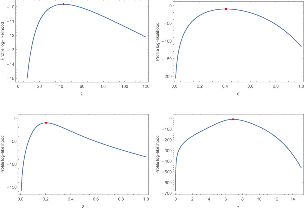

Fig. 3

Plots of the profile-likelihood functions for the four parameters for glass fibers data.

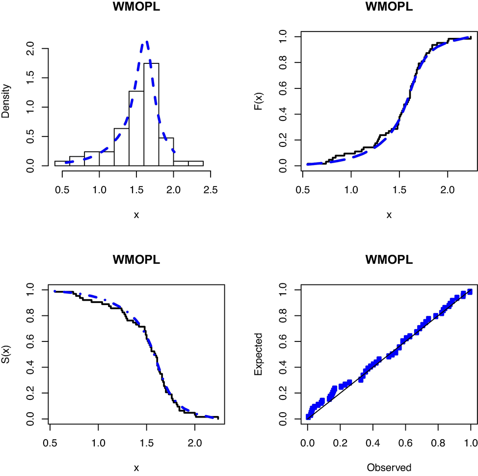
Histogram of glass fibers data with the fitted WMOPL PDF, CDF, SF and P-P plots.

6 Concluding remarks

In this paper, we introduce a new four-parameter distribution called the Weibull Marshall-Olkin power-Lindley (WMOPL) distribution which generalizes some well-known distributions. It is capable of modeling data with decreasing, increasing, J-shaped, reversed-J shaped, unimodal, bathtub, and modified bathtub hazard rate functions. We derive some mathematical properties of the introduced model. The WMOPL parameters are estimated using seven estimation methods. The simulation study explores the performance of these estimators and determines the best estimation method based on partial and overall ranks. Based on this study, the maximum likelihood method outperforms other estimation methods with an overall score of 23. Further, the importance of the WMOPL model is utilized by one real data application from the engineering science. The goodness-of-fit for the data set shows that the introduced model gives better fits in comparison with other well-known Lindley and power-Lindley distributions.

Funding This project is supported by Researchers Supporting Project number (RSP-2020/156) King Saud University, Riyadh, Saudi Arabia.

Acknowledgement

The authors would like to thank the Editor and two referees for their constructive comments that improved the final version of the paper. This work was supported by King Saud University (KSU). The first author, therefore, gratefully acknowledges the KSU for technical and financial support.

Declaration of Competing Interest

The authors declare that they have no known competing financial interests or personal relationships that could have appeared to influence the work reported in this paper.

References

Afify A.Z., Alizadeh M., . The odd Dagum family of distributions: properties and applications. Journal of Applied Probability and Statistics. 2020;15:45-72.
[Google Scholar]
Afify A.Z., Mohamed O.A., . A new three-parameter exponential distribution with variable shapes for the hazard rate: estimation and applications. Mathematics. 2020;8(1):135.
[Google Scholar]
Afify A.Z., Cordeiro G.M., Nadarajah S., Yousof H.M., Ozel G., Nofal Z.M., Altun E., . The complementary geometric transmuted-G family of distributions: model, properties and application. Hacettepe Journal of Mathematics and Statistics. 2016;47(5):1348-1374.
[Google Scholar]
Afify A.Z., Gemeay A.M., Ibrahim N.A., . The heavy-tailed exponential distribution: Risk measures, estimation, and application to actuarial data. Mathematics. 2020;8(8):1276.
[Google Scholar]
Afify A.Z., Nassar M., Cordeiro G.M., Kumar D., . The Weibull Marshall-Olkin Lindley distribution: properties and estimation. Journal of Taibah University for Science. 2020;14(1):192-204.
[Google Scholar]
Al-Babtain A.A., Ahmed A.H.N., Afify A.Z., . A new discrete analog of the continuous lindley distribution, with reliability applications. Entropy. 2020;22:603.
[Google Scholar]
Al-Babtain A.A., Gemeay A.M., Afify A.Z., . Estimation methods for the discrete Poisson-Lindley and discrete Lindley distributions with actuarial measures and applications in medicine. Journal of King Saud University-Science. 2021;33(2):101224
[Google Scholar]
Alizadeh, M., K MirMostafaee, S.M.T., Altun, E., Ozel, G., Khan Ahmadi, M., 2017a. The odd log-logistic Marshall-Olkin power Lindley distribution: Properties and applications. Journal of Statistics and Management Systems, 20(6):1065–1093.
Alizadeh M., Ozel G., Altun E., Abdi M., Hamedani G.G., . The odd log-logistic Marshall-Olkin Lindley model for lifetime data. Journal of Statistical Theory and Applications. 2017;16(3):382-400.
[Google Scholar]
Alizadeh, M., Altun, E., Afify, A.Z., Gamze, O., 2018. The extended odd Weibull-G family: properties and applications. Communications Faculty of Sciences University of Ankara Series A1 Mathematics and Statistics, 68(1), 161–186.
Al-Mofleh H., Afify A.Z., Ibrahim N.A., . A new extended two-parameter distribution: Properties, estimation methods, and applications in medicine and geology. Mathematics. 2020;8(9):1578.
[Google Scholar]
Alzaatreh A., Lee C., Famoye F., . A new method for generating families of continuous distributions. Metron. 2013;71:63-79.
[Google Scholar]
Asgharzadeh A., Nadarajah S., Sharafi F., . Weibull Lindley distribution. REVSTAT. Statistical Journal. 2018;16:87-113.
[Google Scholar]
Cordeiro G., Ortega E., Ramires T., . A new generalized Weibull family of distributions: mathematical properties and applications. Journal of Statistical Distributions and Applications. 2015;2:1-25.
[Google Scholar]
Ghitany M.E., Atieh B., Nadarajah S., . Lindley distribution and its application. Mathematics and Computers in Simulation. 2008;78(4):493-506.
[Google Scholar]
Ghitany M.E., Alqallaf F., Al-Mutairi D.K., Husain H.A., . A two-parameter weighted Lindley distribution and its applications to survival data. Mathematics and Computers in Simulation. 2011;81(6):1190-1201.
[Google Scholar]
Ghitany M.E., Al-Mutairi D.K., Balakrishnan N., Al-Enezi L.J., . Power Lindley distribution and associated inference. Computational Statistics & Data Analysis. 2013;64:20-33.
[Google Scholar]
Hibatullah R., Widyaningsih Y., Abdullah S., . Marshall-olkin extended power lindley distribution with application. Jurnal Riset dan Aplikasi Matematika. 2018;2:84-92.
[Google Scholar]
Korkmaz M., Cordeiro G., Yousof H., Pescim R., Afify A., Nadarajah S., . The Weibull Marshall-Olkin family: regression model and applications to censored data. Communications in Statistics – Theory and Methods. 2019;48:4171-4194.
[Google Scholar]
Lindley D., . Fiducial distributions and bayes theorem. Journal of the Royal Statistical Society. 1958;20:102-107.
[Google Scholar]
Mahmoudi E., Zakerzadeh H., . Generalized Poisson-Lindley distribution. Communications in Statistics Theory and Methods. 2010;39(10):1785-1798.
[Google Scholar]
Marshall A.W., Olkin I., . A new method for adding a parameter to a family of distributions with application to the exponential and weibull families. Biometrika. 1997;84(3):641-652.
[Google Scholar]
Merovci F., . Transmuted Lindley distribution. International Journal of Open Problems in Computer Science and Mathematics. 2013;238(1393):1-20.
[Google Scholar]
Merovci, F., Sharma, V.K., 2014a. The beta-Lindley distribution: properties and applications. Journal of Applied Mathematics.
Merovci F., Sharma V.K., . The Kumaraswamy-Lindley distribution: Properties and applications. 2014.
Nadarajah S., Bakouch H.S., Tahmasbi R., . A generalized Lindley distribution. Sankhya B. 2011;73(2):331-359.
[Google Scholar]
Nassar M., Afify A.Z., Shakhatreh M., . Estimation methods of alpha power exponential distribution with applications to engineering and medical data. Pakistan Journal of Statistics and Operation Research 2020:149-166.
[Google Scholar]
Nassar M., Afify A.Z., Shakhatreh M.K., Dey S., . On a new extension of Weibull distribution: Properties, estimation, and applications to one and two causes of failures. Quality and Reliability Engineering International. 2020;36(6):2019-2043.
[Google Scholar]
Oluyede B.O., Yang T., Makubate B., . A new class of generalized power Lindley distribution with applications to lifetime data. Asian Journal of Mathematics and Applications. 2016;2016:1.
[Google Scholar]
Ozel G., Alizadeh M., Cakmakyapan S., Hamedani G.G., Ortega E.M.M., Cancho V.G., . The odd log-logistic Lindley Poisson model for lifetime data. Communications in Statistics-Simulation and Computation. 2017;46(8):6513-6537.
[Google Scholar]
Smith R.L., Naylor J., . A comparison of maximum likelihood and bayesian estimators for the three-parameter Weibull distribution. Journal of the Royal Statistical Society: Series C (Applied Statistics). 1987;36(3):358-369.
[Google Scholar]
Zakerzadeh, H., Dolati, A., 2009. Generalized Lindley distribution.
Zamani H., Ismail N., . Negative binomial-Lindley distribution and its application. Journal of Mathematics and Statistics. 2010;6(1):4-9.
[Google Scholar]

Introduction

Properties of the WMOPL distribution

Linear representation
Quantile function and moments

Methods of estimation

Maximum likelihood estimators
Anderson–Darling and right-tail Anderson–Darling estimators
Cramer-von-Mises estimators
Maximum product of spacing estimators
Least squares and weighted least squares estimators

Simulation study

Engineering application

Concluding remarks

Fulltext Views
5

PDF downloads
0

View/Download PDF
Download Citations

BibTeX
RIS

Show Sections

[1] Afify A.Z., Alizadeh M., . The odd Dagum family of distributions: properties and applications. Journal of Applied Probability and Statistics. 2020;15:45-72.
[Google Scholar]

[2] Afify A.Z., Mohamed O.A., . A new three-parameter exponential distribution with variable shapes for the hazard rate: estimation and applications. Mathematics. 2020;8(1):135.
[Google Scholar]

[3] Afify A.Z., Cordeiro G.M., Nadarajah S., Yousof H.M., Ozel G., Nofal Z.M., Altun E., . The complementary geometric transmuted-G family of distributions: model, properties and application. Hacettepe Journal of Mathematics and Statistics. 2016;47(5):1348-1374.
[Google Scholar]

[4] Afify A.Z., Gemeay A.M., Ibrahim N.A., . The heavy-tailed exponential distribution: Risk measures, estimation, and application to actuarial data. Mathematics. 2020;8(8):1276.
[Google Scholar]

[5] Afify A.Z., Nassar M., Cordeiro G.M., Kumar D., . The Weibull Marshall-Olkin Lindley distribution: properties and estimation. Journal of Taibah University for Science. 2020;14(1):192-204.
[Google Scholar]

[6] Al-Babtain A.A., Ahmed A.H.N., Afify A.Z., . A new discrete analog of the continuous lindley distribution, with reliability applications. Entropy. 2020;22:603.
[Google Scholar]

[7] Al-Babtain A.A., Gemeay A.M., Afify A.Z., . Estimation methods for the discrete Poisson-Lindley and discrete Lindley distributions with actuarial measures and applications in medicine. Journal of King Saud University-Science. 2021;33(2):101224
[Google Scholar]

[8] Alizadeh, M., K MirMostafaee, S.M.T., Altun, E., Ozel, G., Khan Ahmadi, M., 2017a. The odd log-logistic Marshall-Olkin power Lindley distribution: Properties and applications. Journal of Statistics and Management Systems, 20(6):1065–1093.

[9] Alizadeh M., Ozel G., Altun E., Abdi M., Hamedani G.G., . The odd log-logistic Marshall-Olkin Lindley model for lifetime data. Journal of Statistical Theory and Applications. 2017;16(3):382-400.
[Google Scholar]

[10] Alizadeh, M., Altun, E., Afify, A.Z., Gamze, O., 2018. The extended odd Weibull-G family: properties and applications. Communications Faculty of Sciences University of Ankara Series A1 Mathematics and Statistics, 68(1), 161–186.

[11] Al-Mofleh H., Afify A.Z., Ibrahim N.A., . A new extended two-parameter distribution: Properties, estimation methods, and applications in medicine and geology. Mathematics. 2020;8(9):1578.
[Google Scholar]

[12] Alzaatreh A., Lee C., Famoye F., . A new method for generating families of continuous distributions. Metron. 2013;71:63-79.
[Google Scholar]

[13] Asgharzadeh A., Nadarajah S., Sharafi F., . Weibull Lindley distribution. REVSTAT. Statistical Journal. 2018;16:87-113.
[Google Scholar]

[14] Cordeiro G., Ortega E., Ramires T., . A new generalized Weibull family of distributions: mathematical properties and applications. Journal of Statistical Distributions and Applications. 2015;2:1-25.
[Google Scholar]

[15] Ghitany M.E., Atieh B., Nadarajah S., . Lindley distribution and its application. Mathematics and Computers in Simulation. 2008;78(4):493-506.
[Google Scholar]

[16] Ghitany M.E., Alqallaf F., Al-Mutairi D.K., Husain H.A., . A two-parameter weighted Lindley distribution and its applications to survival data. Mathematics and Computers in Simulation. 2011;81(6):1190-1201.
[Google Scholar]

[17] Ghitany M.E., Al-Mutairi D.K., Balakrishnan N., Al-Enezi L.J., . Power Lindley distribution and associated inference. Computational Statistics & Data Analysis. 2013;64:20-33.
[Google Scholar]

[18] Hibatullah R., Widyaningsih Y., Abdullah S., . Marshall-olkin extended power lindley distribution with application. Jurnal Riset dan Aplikasi Matematika. 2018;2:84-92.
[Google Scholar]

[19] Korkmaz M., Cordeiro G., Yousof H., Pescim R., Afify A., Nadarajah S., . The Weibull Marshall-Olkin family: regression model and applications to censored data. Communications in Statistics – Theory and Methods. 2019;48:4171-4194.
[Google Scholar]

[20] Lindley D., . Fiducial distributions and bayes theorem. Journal of the Royal Statistical Society. 1958;20:102-107.
[Google Scholar]

[21] Mahmoudi E., Zakerzadeh H., . Generalized Poisson-Lindley distribution. Communications in Statistics Theory and Methods. 2010;39(10):1785-1798.
[Google Scholar]

[22] Marshall A.W., Olkin I., . A new method for adding a parameter to a family of distributions with application to the exponential and weibull families. Biometrika. 1997;84(3):641-652.
[Google Scholar]

[23] Merovci F., . Transmuted Lindley distribution. International Journal of Open Problems in Computer Science and Mathematics. 2013;238(1393):1-20.
[Google Scholar]

[24] Merovci, F., Sharma, V.K., 2014a. The beta-Lindley distribution: properties and applications. Journal of Applied Mathematics.

[25] Merovci F., Sharma V.K., . The Kumaraswamy-Lindley distribution: Properties and applications. 2014.

[26] Nadarajah S., Bakouch H.S., Tahmasbi R., . A generalized Lindley distribution. Sankhya B. 2011;73(2):331-359.
[Google Scholar]

[27] Nassar M., Afify A.Z., Shakhatreh M., . Estimation methods of alpha power exponential distribution with applications to engineering and medical data. Pakistan Journal of Statistics and Operation Research 2020:149-166.
[Google Scholar]

[28] Nassar M., Afify A.Z., Shakhatreh M.K., Dey S., . On a new extension of Weibull distribution: Properties, estimation, and applications to one and two causes of failures. Quality and Reliability Engineering International. 2020;36(6):2019-2043.
[Google Scholar]

[29] Oluyede B.O., Yang T., Makubate B., . A new class of generalized power Lindley distribution with applications to lifetime data. Asian Journal of Mathematics and Applications. 2016;2016:1.
[Google Scholar]

[30] Ozel G., Alizadeh M., Cakmakyapan S., Hamedani G.G., Ortega E.M.M., Cancho V.G., . The odd log-logistic Lindley Poisson model for lifetime data. Communications in Statistics-Simulation and Computation. 2017;46(8):6513-6537.
[Google Scholar]

[31] Smith R.L., Naylor J., . A comparison of maximum likelihood and bayesian estimators for the three-parameter Weibull distribution. Journal of the Royal Statistical Society: Series C (Applied Statistics). 1987;36(3):358-369.
[Google Scholar]

[32] Zakerzadeh, H., Dolati, A., 2009. Generalized Lindley distribution.

[33] Zamani H., Ismail N., . Negative binomial-Lindley distribution and its application. Journal of Mathematics and Statistics. 2010;6(1):4-9.
[Google Scholar]

Modeling engineering data using extended power-Lindley distribution: Properties and estimation methods

Abstract

Keywords

Anderson–Darling estimation

Maximum likelihood estimation

Maximum product of spacing

Moments

Power-Lindley distribution

1 Introduction

2 Properties of the WMOPL distribution

2.1 Linear representation

2.2 Quantile function and moments

3 Methods of estimation

3.1 Maximum likelihood estimators

3.2 Anderson–Darling and right-tail Anderson–Darling estimators

3.3 Cramer-von-Mises estimators

3.4 Maximum product of spacing estimators

3.5 Least squares and weighted least squares estimators

4 Simulation study

5 Engineering application

6 Concluding remarks

Acknowledgement

Declaration of Competing Interest

References

Suggested read for related articles: