Translate this page into:
MLPG method based on moving kriging interpolation for solving convection–diffusion equations with integral condition
⁎Corresponding author. anirut.lua@kmutt.ac.th (A. Luadsong)
-
Received: ,
Accepted: ,
This article was originally published by Elsevier and was migrated to Scientific Scholar after the change of Publisher.
Peer review under responsibility of King Saud University.
Abstract
A formulation of the meshless local Petrov–Galerkin (MLPG) method based on the moving kriging interpolation (MK) is presented in this paper. The method is used for solving time-dependent convection–diffusion equations in two-dimensional spaces with the Dirichlet, Neumann, and non-local boundary conditions on a square domain. The method is developed based on the moving kriging interpolation method for constructing shape functions which have the Kronecker delta property. In the method, the test function in each sub-domain is chosen as the indicator function. The Crank–Nicolson method is chosen for temporal discretization. Two test problems are presented which demonstrate the easiness and accuracy of this method as shown by the relative error.
Keywords
Convection–diffusion equations
Crank–Nicolson
Moving kriging interpolation
MLPG
Integral condition
1 Introduction
In recent decades, meshless method in mathematical modeling has attracted much attention, due to their flexibility in solving practical science and engineering problems. The meshless method has been developed and achieved remarkable progress in mathematical modeling and related fields. The main reason for interest in meshless method is it can save computational time because no mesh is needed. They can easily produce high accuracy, since in areas where more refinement is required; nodes can quite easily be added. In addition, they can easily construct high-order shape functions. They can easily solve large deformation and strong nonlinear problem. The connectivity among the nodes is generated as a part of the computation and can change with time.
Based on the form of system equation, the meshfree methods are classified into three categories. The first category covers the meshfree methods based on strong forms of system equations, in which discretization is performed directly from the governing differential equations, such as the general finite difference method (Liszka and Orkisz, 1980), the smooth particle hydrodynamic (SPH) method (Liu and Liu, 2003; Lucy, 1977), and other meshfree collocation methods. The second category includes meshfree methods based on weak forms of system equations, such as the element-free Galerkin (EFG) method (Belytschko et al., 1994), the meshless local Petrov–Galerkin (MLPG) method (Atluri and Zhu, 1998; Atluri and Lin, 2000; Abbasbandy and Shirzadi, 2011; Mirzaei, 2010; Mahmoodabadi et al., 2011), the point interpolation method (PIM) (Liu, 2002; Liu and Gu, 2001), etc. The third category concerns meshfree methods based on the combination of weak and strong forms, such as the meshfree weak–strong-form (MWS) method. The major difference in these meshless methods is in the choice of interpolation techniques.
The MLPG method was first discovered by Atluri and Zhu (1998). Meshless local Petrov–Galerkin (MLPG) method is a truly meshless method. This method is based on a weak form computed over a local sub-domain and the moving least squares (MLS) approximation. The MLPG method is one of the most viable methods in which the MLS approach is used to construct the shape functions. Although the MLPG method has been applied to many problems, there exists an inconvenience or disadvantage when using the MLPG because of the difficulty in implementing essential boundary conditions. This is because the MLS shape functions lack the Kronecker delta property. Therefore the MK interpolation method (Yimnak and Luadsong, 2014; Kaewumpai and Luadsong, 2014) has been proposed to overcome this problem. It uses the nodal values in the local support domain to construct shape functions with the Kronecker delta property. The MK interpolation method works well for practical problems.
Finding numerical solutions with non-local boundary conditions is important in applications such as chemical diffusion, heat conduction processes, population dynamics thermoelasticity, medical science, electrochemistry and control theory. Because of the complex problems, some analytic solutions are difficult to find in the sense of boundary conditions and geometrical shapes. So, recently much attention has been paid in the literature to the analysis and implementation of accurate methods for the numerical solution of time-dependent partial differential equations with non-local boundary conditions. Abbasbandy and Shirzadi (2010) researched on the MPLG method for the two-dimensional diffusion equation with the Neumann boundary condition and non-classical boundary condition, and a meshless method for the two-dimensional diffusion equation with an integral condition. Mohyud-Din and Yildirim (2010) employed the homotopy analysis method (HAM) for the solutions of two-dimensional diffusion equations subject to non-standard boundary specifications. The HAM method does not need transformation techniques, linearization and discretization. The approximate solutions by the HAM method were compared with exact solutions. It was shown that the method is reliable, efficient and requires less computation. Sajavicius (2013) researched optimization, conditioning and accuracy of radial basis function method for partial differential equations with nonlocal boundary conditions in case of two-dimensional Poisson equation. Techapirom and Luadsong (2013) have used an MLPG method to study the two-dimensional heat equation with Dirichlet, Neumann and non-local boundary conditions in a square domain. Their study demonstrated the good accuracy of the proposed method and indicates that it can be easily extrapolated to other problems. Sataprahm and Luadsong (2014) have used the Meshless Local Petrov–Galerkin (MLPG) method for the incompressible Navier–Stokes equations. The numerical examples presented the local symmetric weak form (LSWF) and the local unsymmetric weak form (LUSWF) with a classical Gaussian weight and an improved Gaussian weight on both regular and irregular nodes is demonstrated. It is found that LSWF1 with a classical Gaussian weight order 2 gives the most accurate result. Goodrich (2015) considers the coupled systems of boundary value problems with nonlocal boundary conditions. The result shows that this system can possess at least one positive solution even if no growth conditions. Islam et al. (2015) present two numerical methods that are analyzed for the solution of two-dimensional Poisson equation with two different types of nonlocal boundary conditions. The first numerical method is a collocation method based on Haar wavelet whereas the second numerical method is a meshless method based on different types of radial basis functions (RBFs). A two-point boundary condition and an integral boundary condition are the two types of nonlocal boundary conditions considered in the present work. Two numerical results have shown that the accuracy and efficiency wise performance is confirmed through application of the algorithms on the benchmark tests.
The purpose of this article is to present a very efficient MLPG based on MK interpolation for solving the two-dimensional time-dependent convection–diffusion equation with integral conditions. To deal with time derivatives, using the Crank–Nicolson implicit method. The solution is approximated by the MK interpolation method which holds the Kronecker delta property, thereby enhancing the nodal shape construction accuracy. It was shown that the method is reliable and efficient. Two test problems are presented illustrating the easiness and accuracy of this method as shown by the relative error.
2 Moving kriging interpolation method
The kriging interpolation is well-known geostatic technique for spatial interpolation in geology and mining (Lucy, 1977). The formulation of the construction of meshless shape function by MK interpolation is introduced briefly in the following. Similar to the MLS approximation, consider the function
defined in the domain
discretized by a set of properly scattered nodes
, where
is the total number of nodes in the whole domain. It is assumed that only
nodes surrounding point
have the effect on
. The sub-domain
that encompasses these surrounding nodes is called the interpolation domain of point
. The MK interpolation
at point
is defined as presented in Liu and Gu (2001). Therefore, the formulation of the meshless shape function using MK interpolation is given by:
In which I is a unit matrix of size N × N, and vector
is:
For matrix P with the size N × M, values of the polynomial basis functions at the given set of nodes are collected:
Matrices R and vector
are defined by the following equations:
Similarly, the covariance
can be replaced by
. It can be seen from the foregoing formulations that the values of matrices R and
play important roles in the computation. A simple and frequently- used correlation function is a Gaussian function:
The first-order partial derivatives of the shape function
against the coordinates
can be easily obtained from Eq. (2)
3 Formulation of the moving kriging interpolation for convection–diffusion equation
3.1 Governing equation and boundary conditions
The two-dimensional time-dependent convection–diffusion equation subject to non-local boundary conditions can be written as:
-
–
The non-local boundary condition:
(13) -
–
The essential boundary condition:
(14) -
–
The natural boundary condition:
(15) -
–
The initial condition assumed to be
(16)and the integral condition(17)
3.2 Local weak-forms
In implementation of the present MK interpolation method, a weak form is first constructed over a local sub-domain
bounded by
, where
is located entirely inside the global domain
. Using the local weighted residual technique, the local weak form of Eq. (12) over a local sub-domain
can be written as:
Using
and the divergence theorem, we obtain the following local weak formulation (LWF):
In general, the boundary
of the local sub-domain
may intersect with the boundary of the global domain
. Therefore,
where,
is a part of
. By imposing the natural boundary condition, we obtain:
The test function in each sub-domain is chosen as the indicator function.
3.3 Discretization of the weak form
As a known test function is used in the LWF, the use of the LWF for one point (and hence for one local domain) will yield only one linear equation involving . Note that the trial function within the sub-domain , in the MK approximation, is determined by the fictitious nodal values within the domain of definition for all points falling within . The LWF in Eq. (22) gives one algebraic equation relating all these . Thus, we obtain as many equations as the number of nodes. Therefore, we need as many local domains as the number of nodes in the global domain to obtain as many equations as the number of unknowns. In the present implementation, the local domain is chosen as a circle, centered at a node .
To obtain the discrete equations from the LWF in Eq. (22), the MK approximation in Eq. (1), is alternatively used to approximate the trial function
. Substituting of Eq. (1) into the LWF Eq. (22) for the entire node, leads to the following discretized system of linear equations:
Eq. (23) can be written in the matrix form as follows:
Setting a time-stepping scheme to overcome the time derivative and applying the Crank–Nicolson technique of approximation to Eq. (24) yields:
Assuming that
, for
and
are known, our aim is to compute
for
and
. Now, we have
unknowns, so to compute these unknowns we need one equation, which can be obtained from the non-local boundary condition from Eq. (17). Substituting trial function Eq. (1), we obtain:
For nodes on the natural, essential and non-local boundaries, we present an algorithm to impose boundary conditions as follows:
-
–
For node is on the natural boundary condition,
(33) -
–
For node is on the essential boundary condition,
(34) -
–
For node is on the non-local boundary condition,
(35)
4 Numerical examples
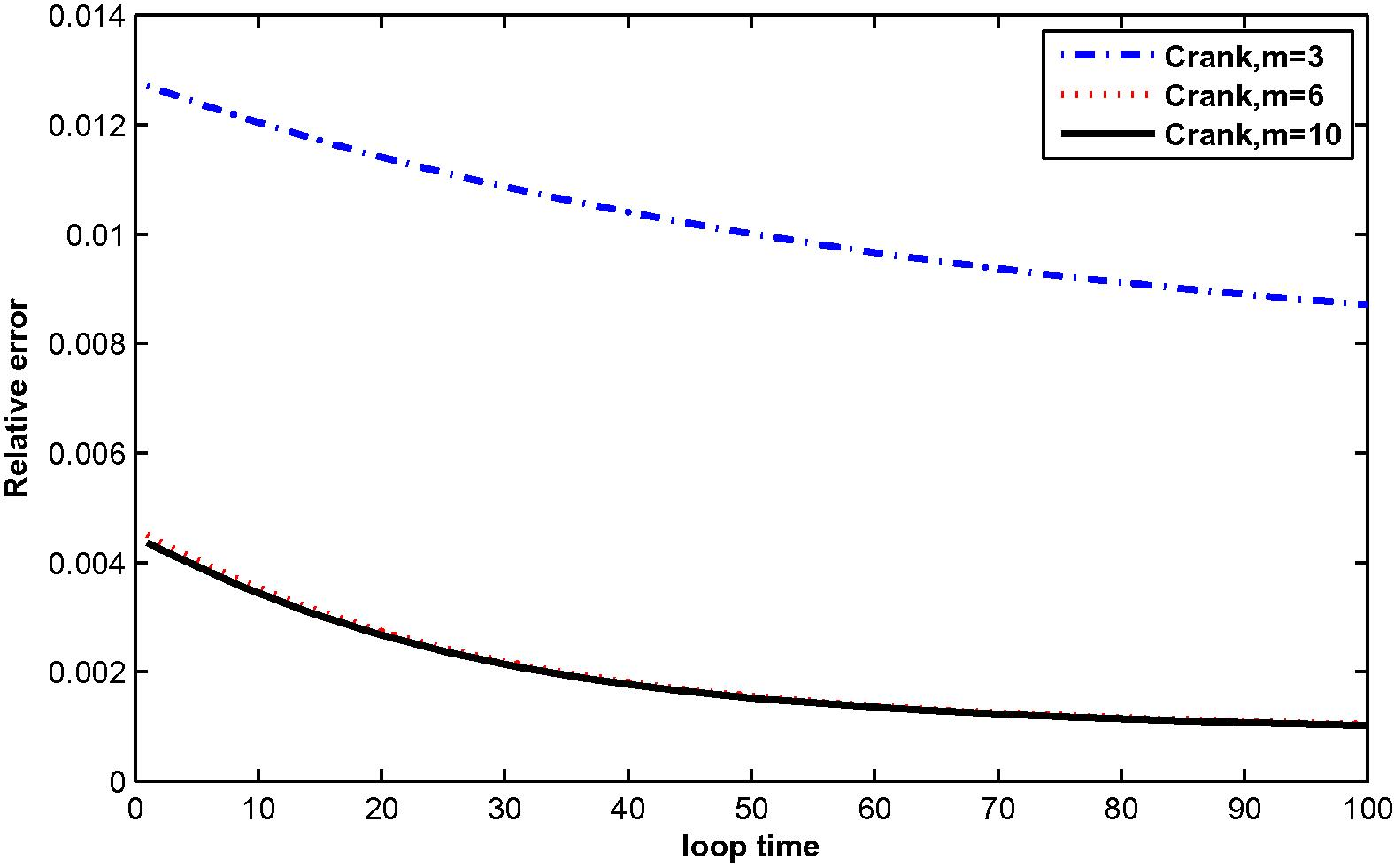
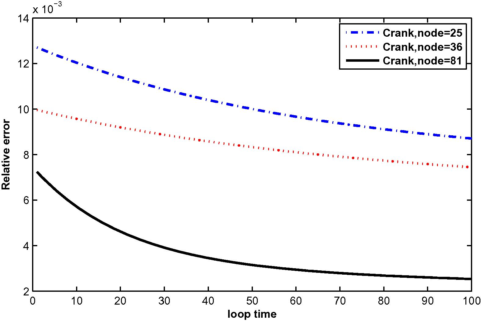
In the computation, problems are considered in a unit square domain given by . The flow is unidirectional and constant with velocity components and . The diffusivity coefficient is 1. The radius of the local sub-domain for each node is chosen as , with is the distance between two consecutive nodes in each direction. The results are obtained for and for several time levels with . The numbers of complete monomial basis (M) are 3, 6 and 10 and the numbers of nodal points (N) are 25, 36 and 81. The exact solutions are known for these problems and are used to test the accuracy of these numerical schemes. The numerical results in these tables show that the method converges by increasing the number of nodal points, and increasing the number of monomial basis for a fixed number of nodal points enhance accuracy.
4.1 Problem 1
We consider the two-dimensional time-dependent convection–diffusion equation with Dirichlet and non-local boundary condition: subject to initial, Dirichlet boundary conditions and non-local boundary conditions:
The exact solution of this problem is:
The source term of this problem is:
The numerical results are shown in Tables 1 and 2, Figs. 1–12.
N/m
3
6
10
25
2.0163e−2
3.1541e-3
2.5064e-3
36
1.7916e-2
2.6715e-3
1.9803e-3
81
6.2939e-3
2.5497e-3
1.5738e-3
N/m
3
6
10
25
8.8847e-3
1.0669e-3
1.0410e-3
36
7.5965e-3
7.2043e-4
6.6892e-4
81
2.5943e-3
6.5504e-4
5.9344e-4
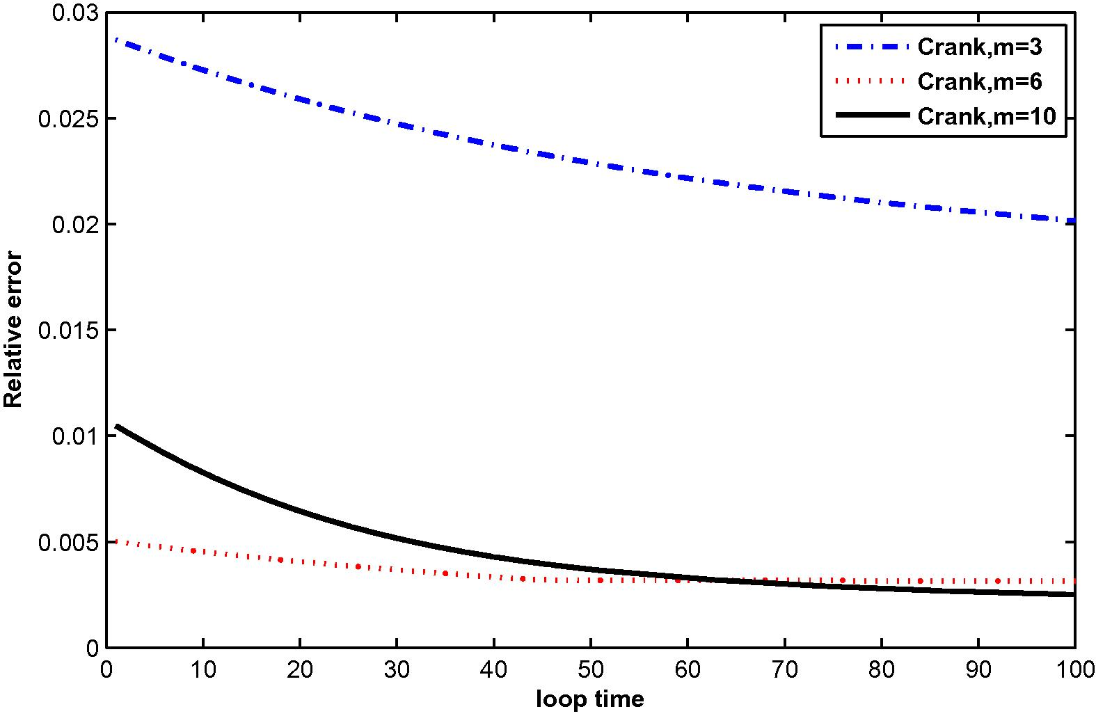
The relative error for
at M = 3, 6 and 10 with N = 25.
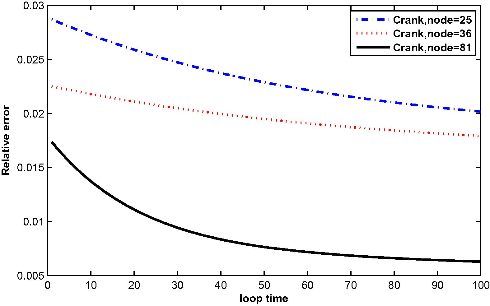
The relative error for
at N = 25, 36 and 81 with M = 3.
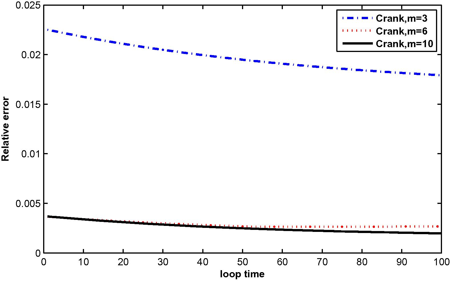
The relative error for
at M = 3, 6 and 10 with N = 36.
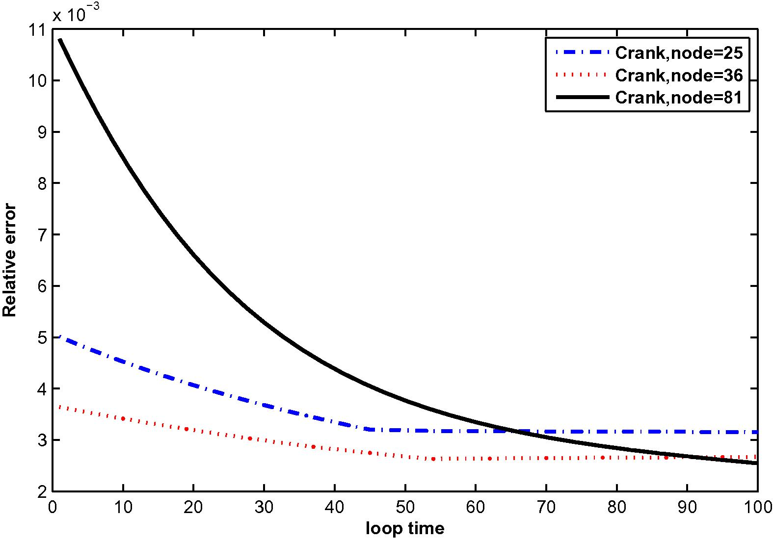
The relative error for
at N = 25, 36 and 81 with M = 6.
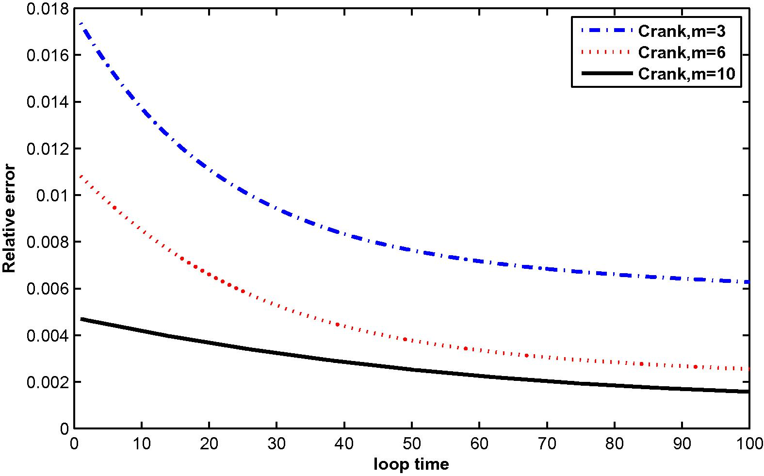
The relative error for
at M = 3, 6 and 10 with N = 81.
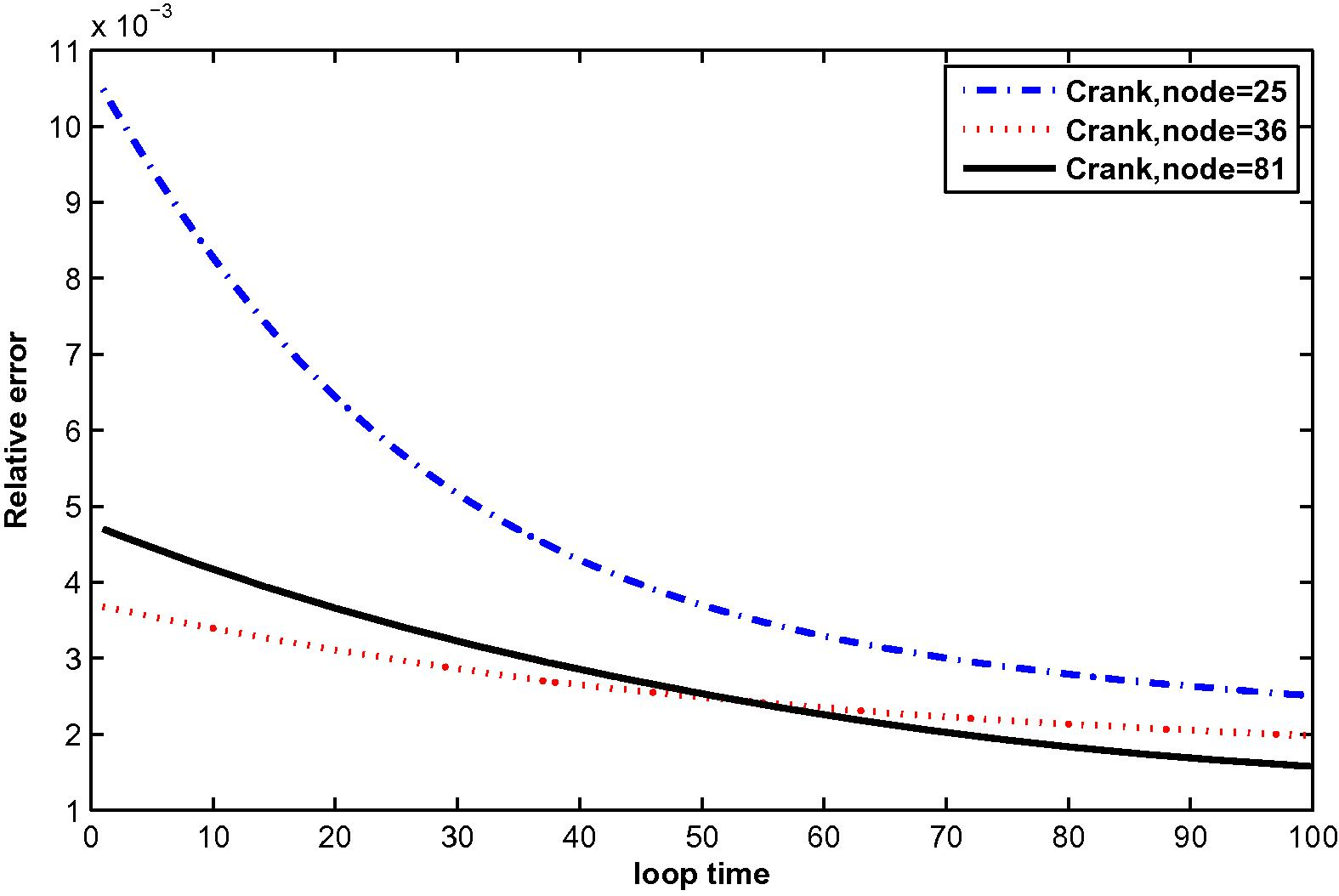
The relative error for
at N = 25, 36 and 81 with M = 10.
The relative error for
at M = 3, 6 and 10 with N = 25.
The relative error for
at N = 25, 36 and 81 with M = 3.
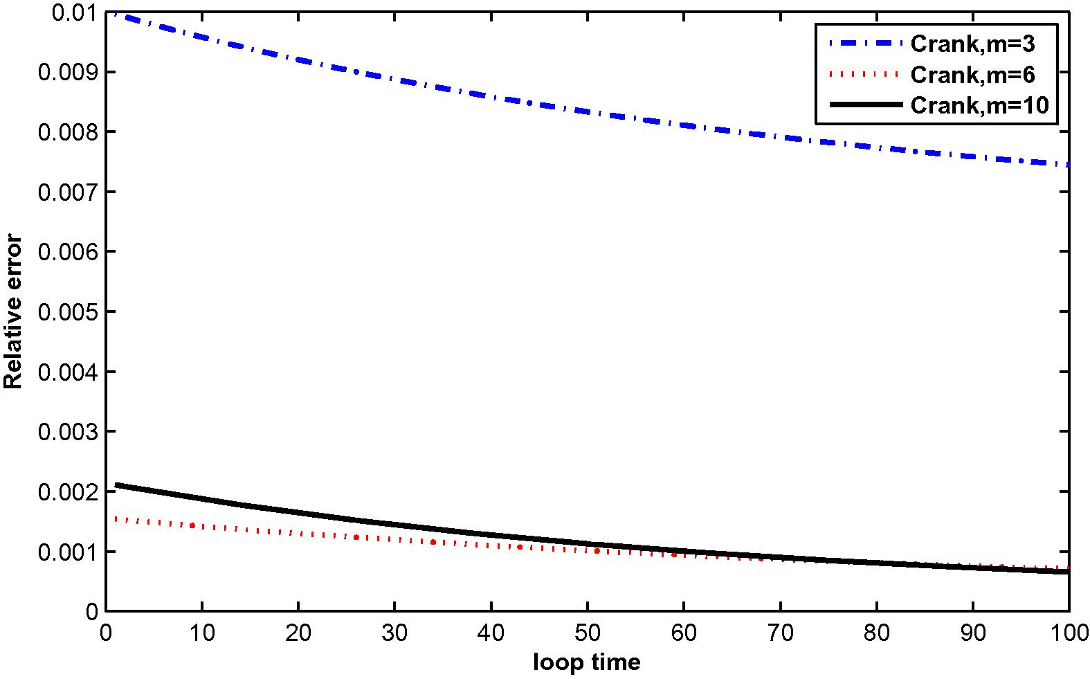
The relative error for
at M = 3, 6 and 10 with N = 36.
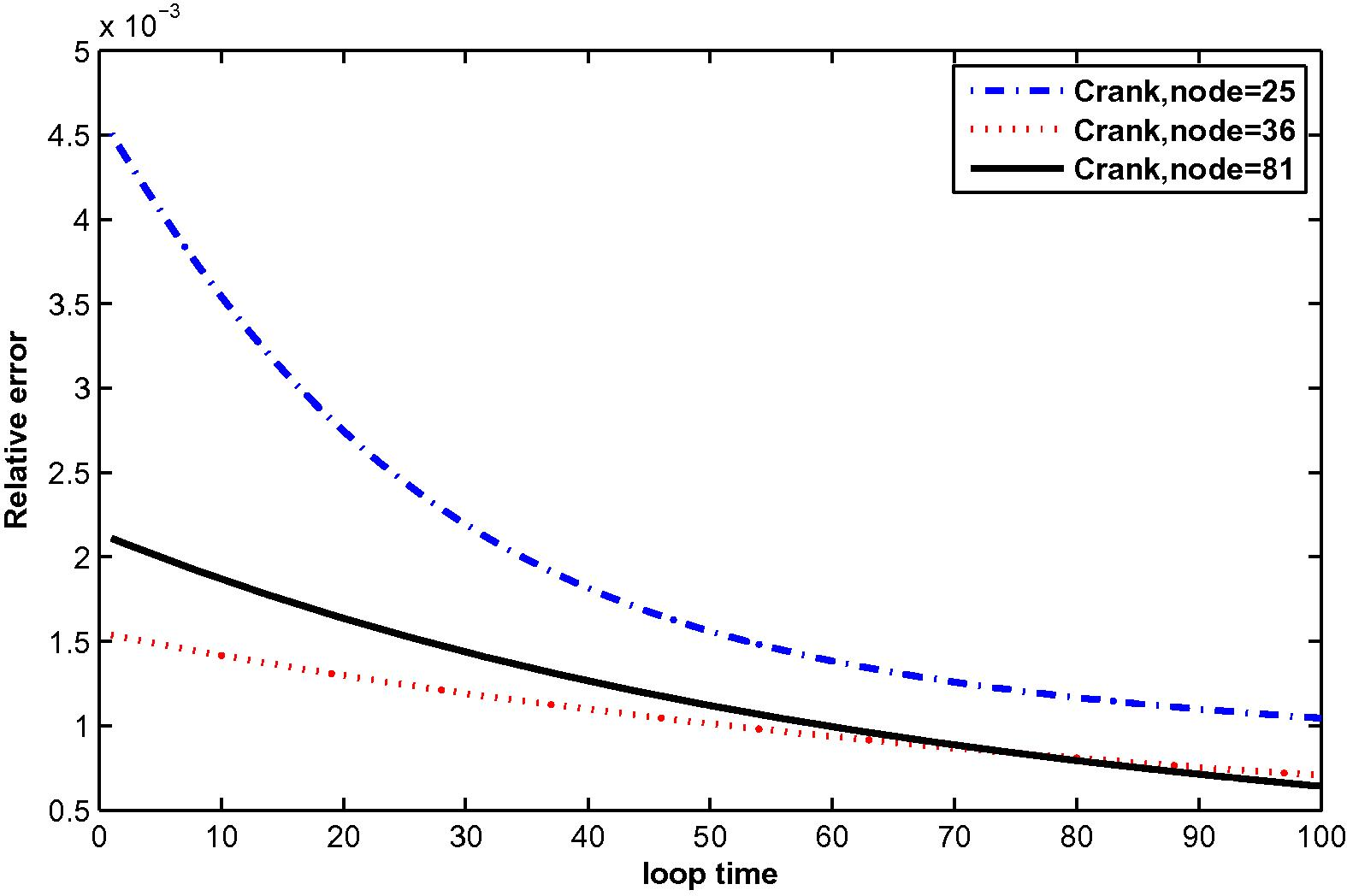
The relative error for
at N = 25, 36 and 81 with M = 6.
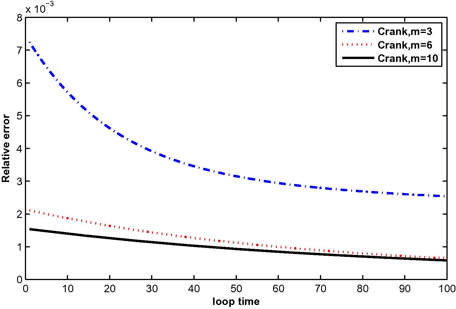
The relative error for
at M = 3, 6 and 10 with N = 81.
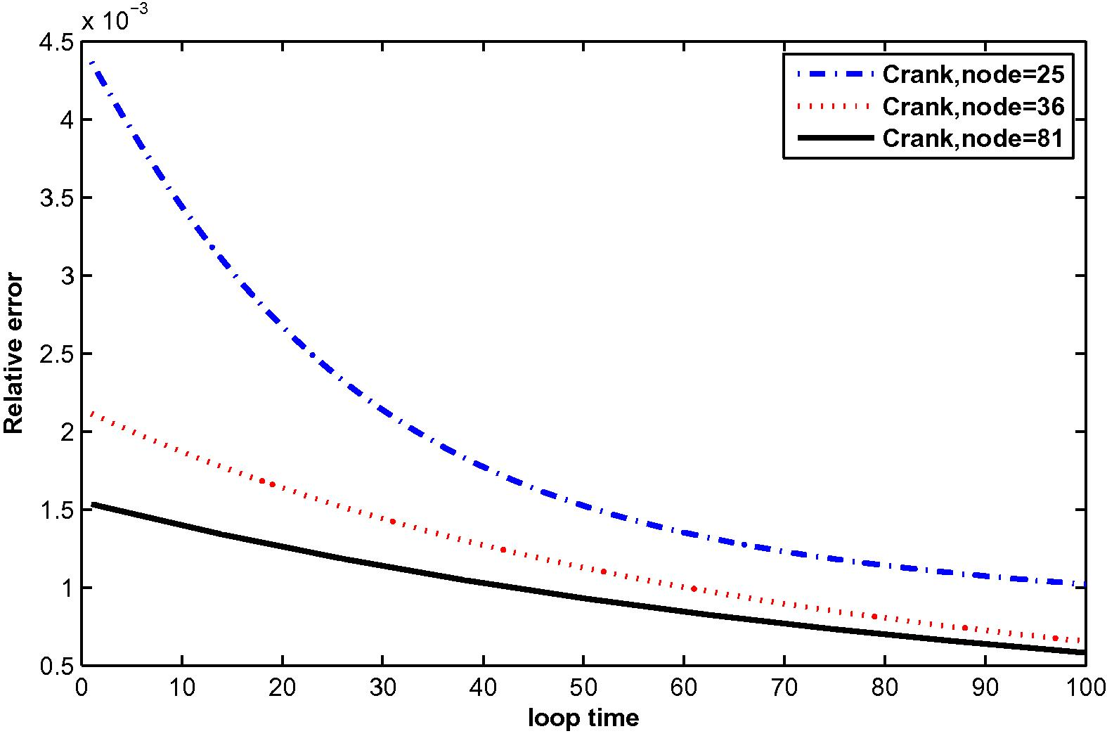
The relative error for
at N = 25, 36 and 81 with M = 10.
4.2 Problem 2
We consider the two-dimensional time-dependent convection–diffusion equation with Dirichlet, Neumann and non-local boundary condition: subject to initial, Dirichlet boundary condition, Neumann boundary condition and non-local boundary condition:
The exact solution of this problem is:
The source term of this problem is:
The numerical results are shown in Tables 3 and 4, Figs. 13–24.
N/m
3
6
10
25
1.9372e-2
5.3279e-3
4.4636e-3
36
1.6748e-2
4.8862e-3
2.7373e-3
81
5.8101e-3
2.8265e-3
1.5231e-3
N/m
3
6
10
25
6.1612e-3
1.0348e-3
1.0079e-3
36
2.5005e-3
5.6160e-4
5.4160e-4
81
1.7075e-3
3.1049e-4
3.0039e-4
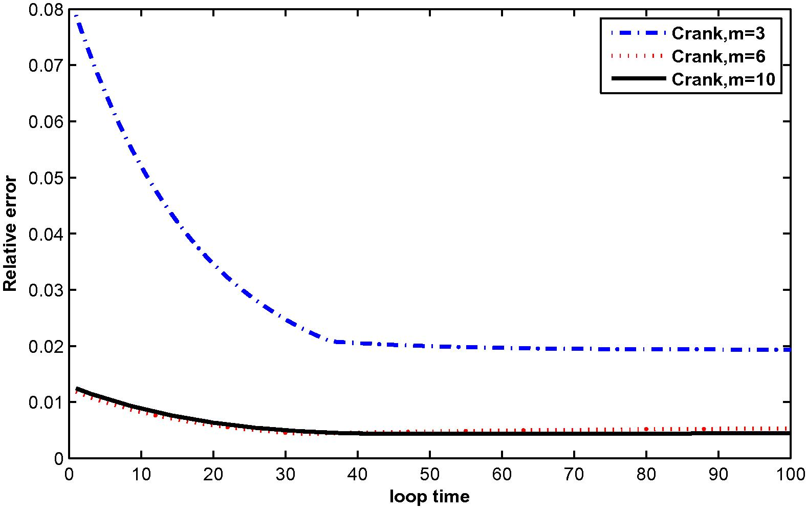
The relative error for
at M = 3, 6 and 10 with N = 25.
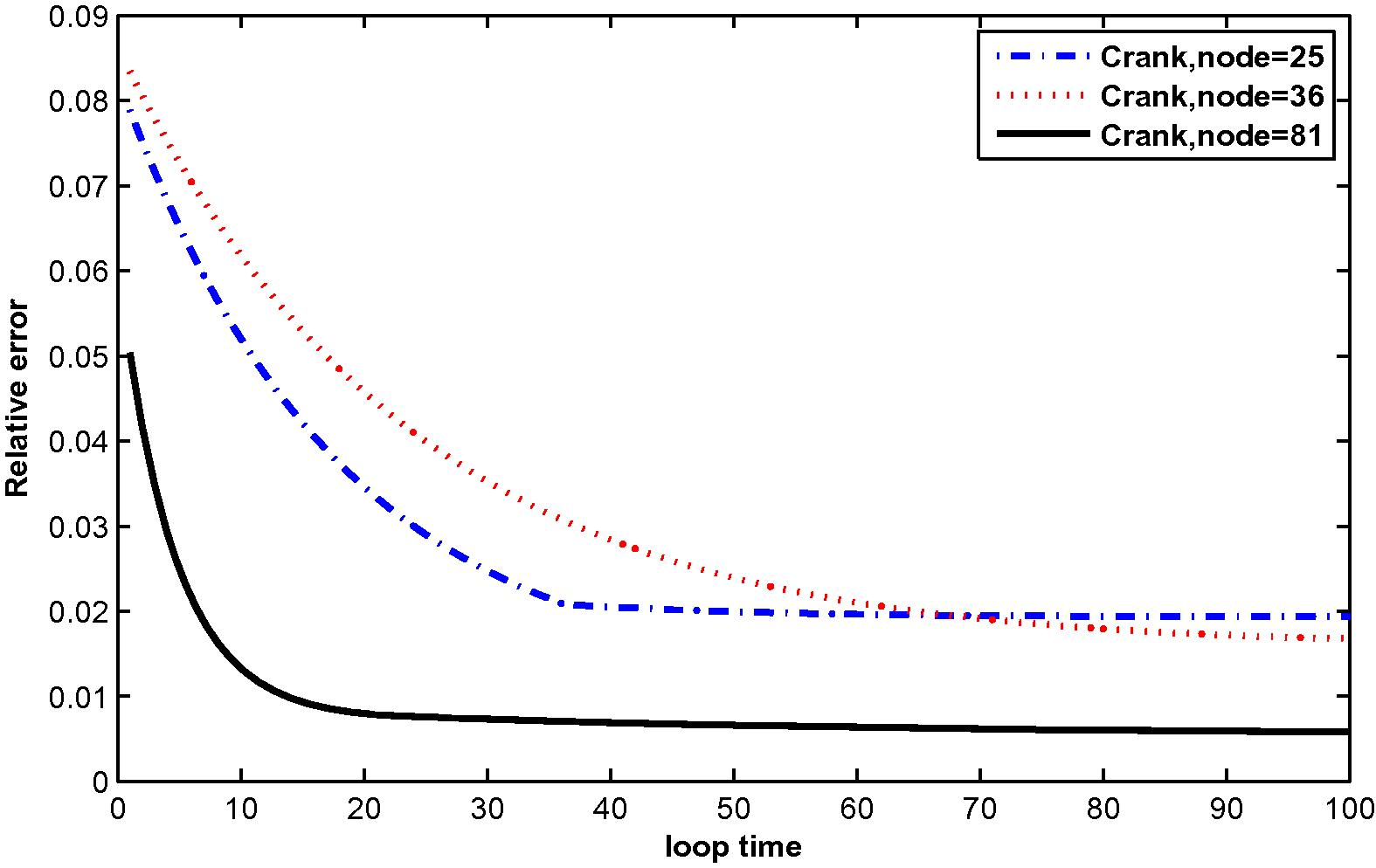
The relative error for
at N = 25, 36 and 81 with M = 3.
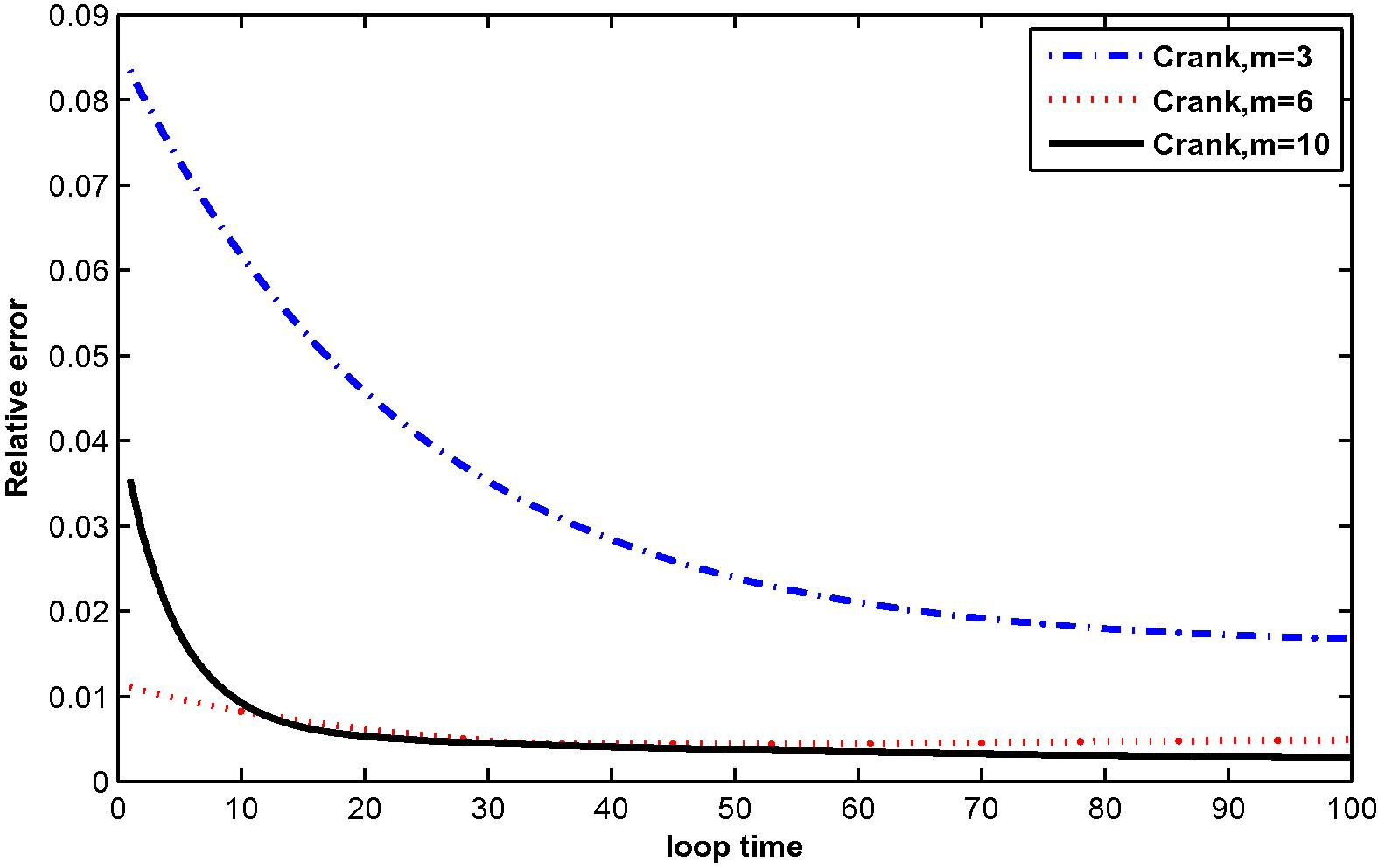
The relative error for
at M = 3, 6 and 10 with N = 36.
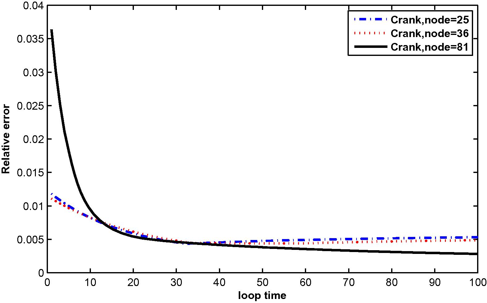
The relative error for
at N = 25, 36 and 81 with M = 6.
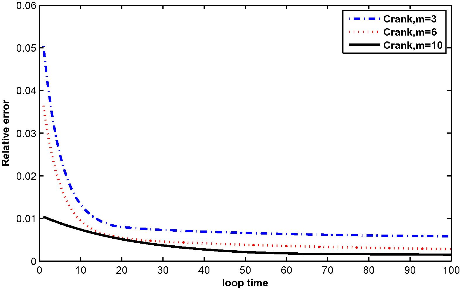
The relative error for
at M = 3, 6 and 10 with N = 81.
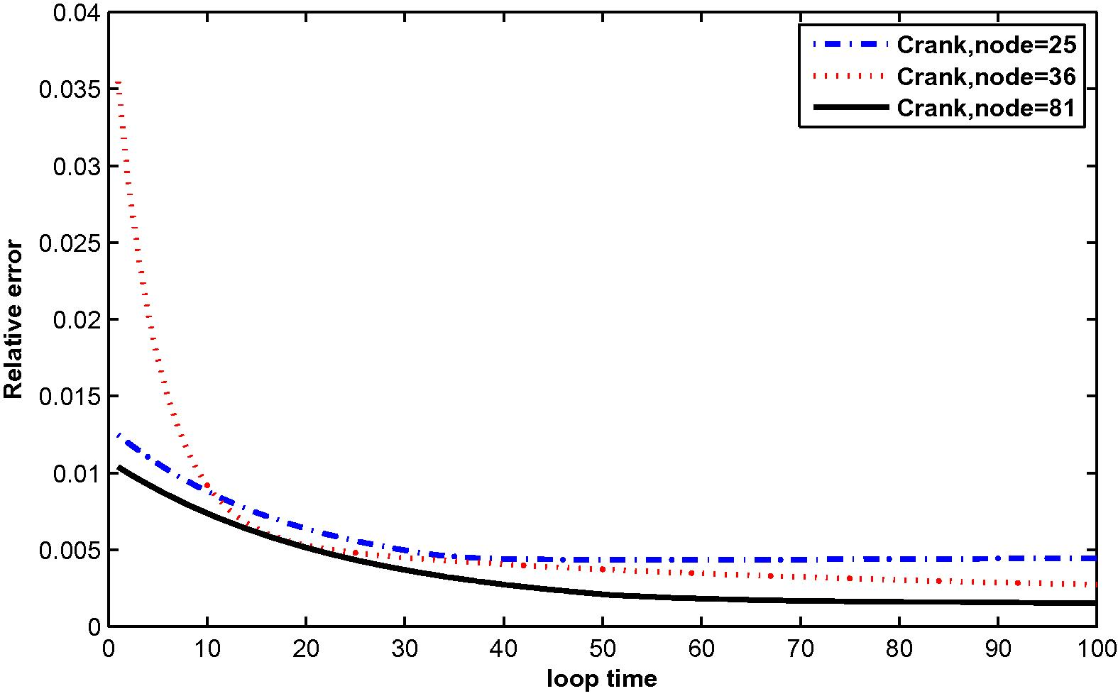
The relative error for
at
=25, 36 and 81 with M = 10.
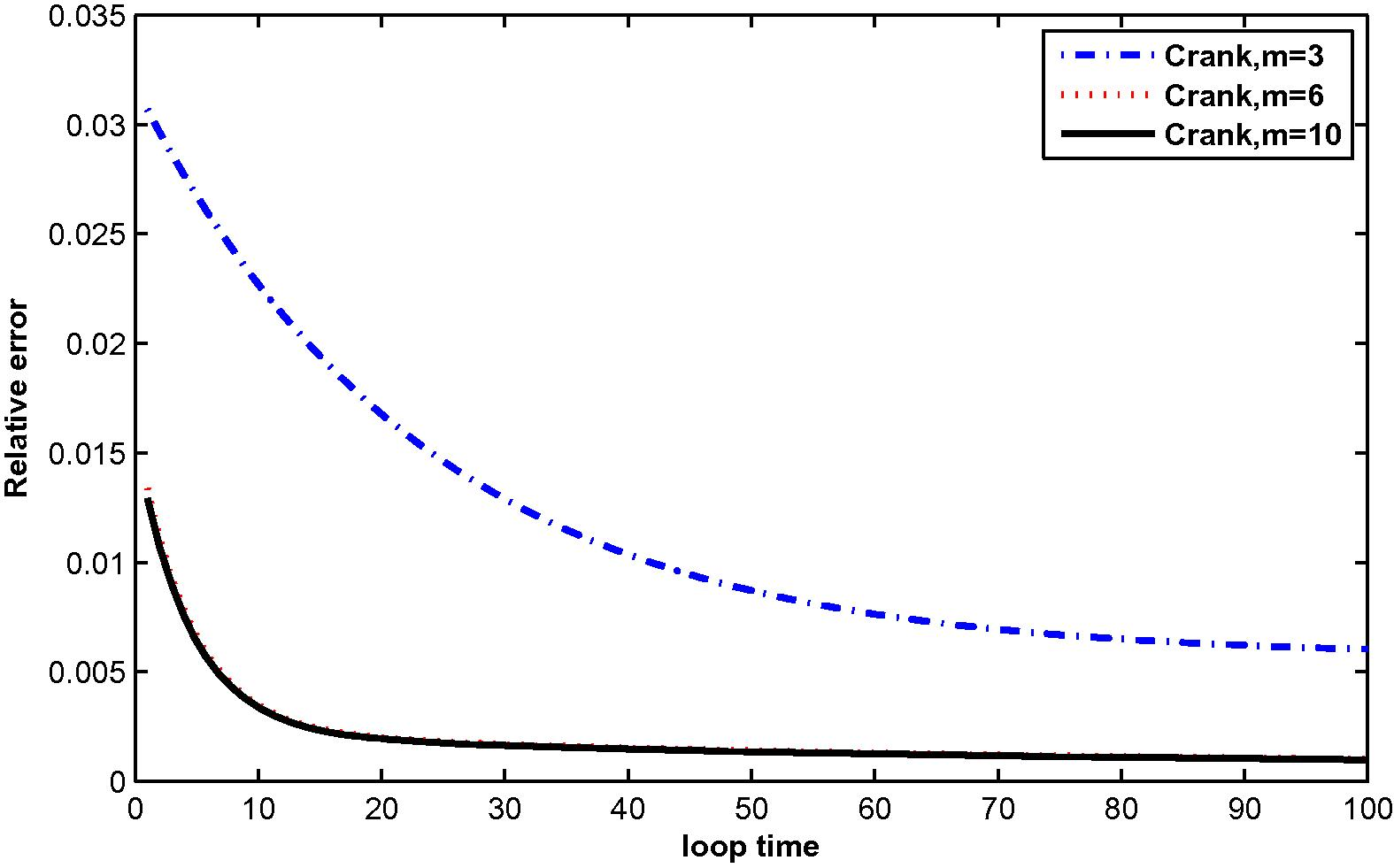
The relative error for
at M = 3, 6 and 10 with N = 25.
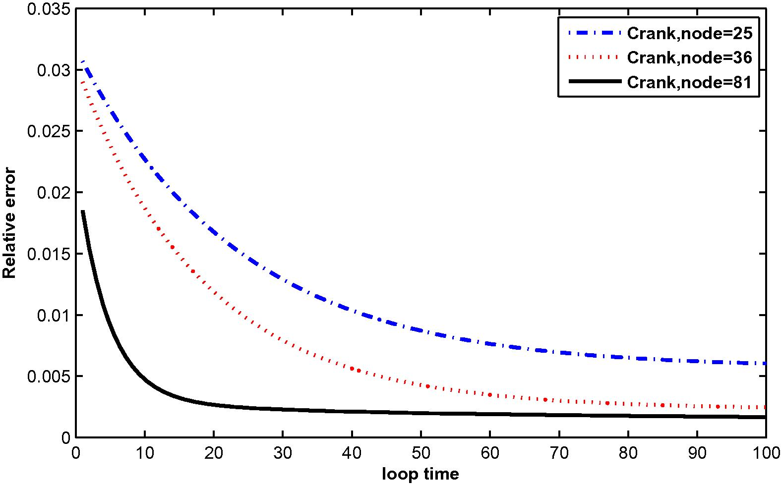
The relative error for
at N = 25, 36 and 81 with M = 3.
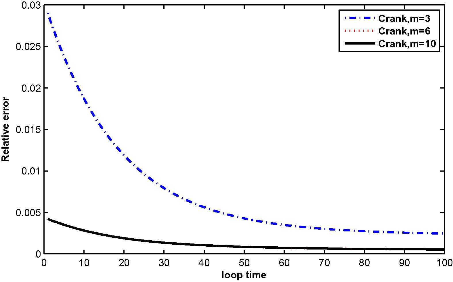
The relative error for
at M = 3, 6 and 10 with N = 36.
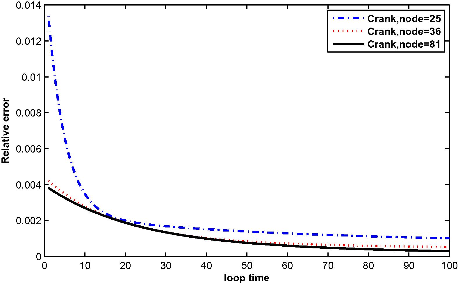
The relative error for
at N = 25, 36 and 81 with M = 6.
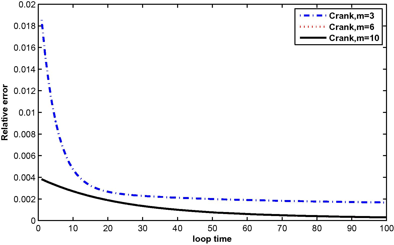
The relative error for
at M = 3, 6 and 10 with N = 81.
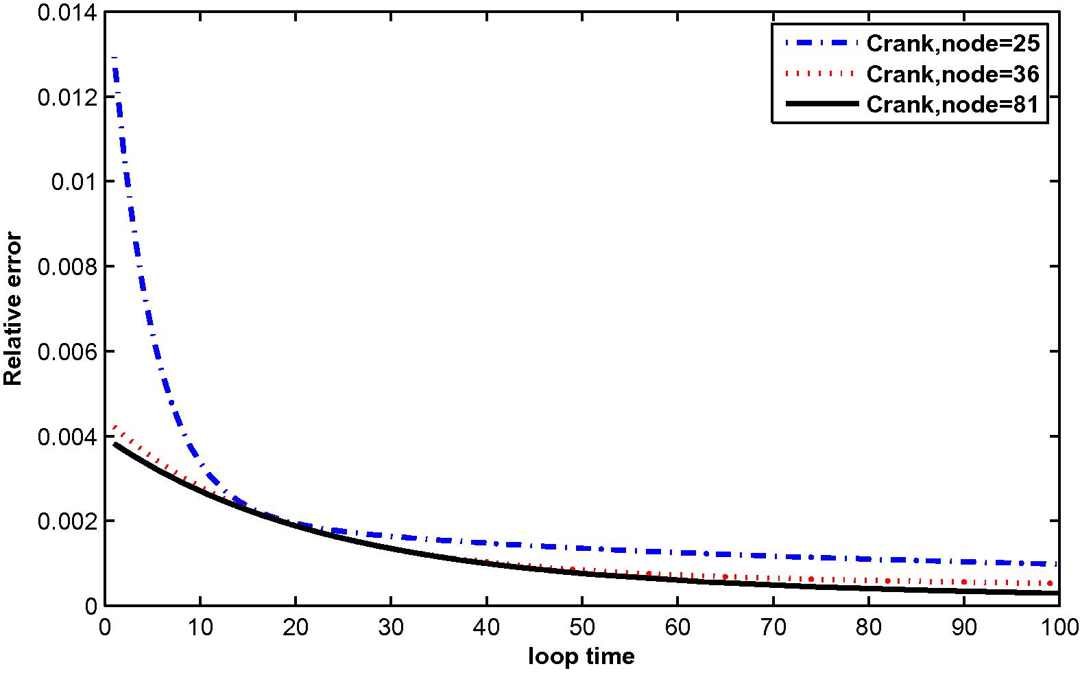
The relative error for
at N = 25, 36 and 81 with M = 10.
5 Conclusions
A formulation of meshless local Petrov–Galerkin (MLPG) has been presented in the present work. We have proposed an idea of MK interpolation demonstrating how it can be used to construct the meshless shape functions for solving the two-dimensional time-dependent convection–diffusion equation with integral conditions. To deal with time derivatives, the Crank–Nicolson implicit method was used. The key feature of the MK interpolation is that the shape function possesses the Kronecker delta property which makes it easy to directly impose Dirichlet boundary conditions. The numerical results show a decrease in relative error with increasing number of nodal points. Similarly, the relative error decreases when the size of the monomial basis increases. Moreover, it can be concluded that the numerical results of two test problems have been used to verify the efficiency, easiness and accuracy of the method.
Acknowledgements
This research is partially supported by the Science Achievement Scholarship of Thailand in Mathematics.
References
- A meshless method for two-dimensional diffusion equation with an integral condition. Eng. Anal. Bound. Elem.. 2010;34:1031-1037.
- [Google Scholar]
- MLPG method for two-dimensional diffusion equation with Neumann’s and non-classical boundary conditions. Appl. Numer. Math.. 2011;61:170-180.
- [Google Scholar]
- Meshless local Petrov–Galerkin (MLPG) method for convection–diffusion problems. CMES. 2000;1(2):45-60.
- [Google Scholar]
- A new meshless local Petrov–Galerkin (MLPG) approach in computational mechanics. Comput. Mech.. 1998;22:117-127.
- [Google Scholar]
- Coupled systems of boundary value problems with nonlocal boundary conditions. Appl. Math. Lett.. 2015;41:17-22.
- [Google Scholar]
- Numerical solution of two-dimensional elliptic PDEs with nonlocal boundary conditions. Comput. Math. Appl.. 2015;69:180-205.
- [Google Scholar]
- Two-field-variable meshless method based on moving kriging interpolation for solving simply supported thin plates under various loads. J. King Saud Univ. Sci. 2014:1018-3647.
- [Google Scholar]
- The finite difference method on arbitrary irregular grid and its application in applied mechanics. Comput. Struct.. 1980;11:83-95.
- [Google Scholar]
- A point assembly method for stress analysis for two-dimensional solids. Int. J. Solids Struct.. 2002;39:261-276.
- [Google Scholar]
- A point interpolation method for two-dimensional solid. Int. J. Numer. Methods Eng.. 2001;50:937-951.
- [Google Scholar]
- Smoothed Particle Hydrodynamics – A Meshfree Practical Method. Singapore: World Scientific; 2003.
- A numerical approach to testing the fission hypothesis. Astrophys. J.. 1977;82:1013-1024.
- [Google Scholar]
- Meshless local Petrov–Galerkin method for 3D steady-state heat conduction problems. Adv. Mech. Eng. 2011 (10 pages)
- [CrossRef] [Google Scholar]
- Meshless local Petrov–Galerkin (MLPG) approximation to the two dimensional sine-Gordor equation. Appl. Math. Comput.. 2010;233:2737-2754.
- [Google Scholar]
- On two-dimensional diffusion with integral condition. J. King Saud Univ. Sci.. 2010;23(2):121-125.
- [Google Scholar]
- Optimization, conditioning and accuracy of radial basis function method for partial differential equations with nonlocal boundary condition-A case of two-dimensional Poisson equation. Eng. Anal. Bound. Elem.. 2013;37:788-804.
- [Google Scholar]
- The meshless local Petrov–Galerkin method for simulating unsteady incompressible fluid flow. J. Egypt. Math. Soc.. 2014;23(3):501-510.
- [Google Scholar]
- The MLPG with improved weight function for two-dimensional heat equation with non-local boundary condition. J. King Saud Univ. Sci.. 2013;25:341-348.
- [Google Scholar]
- A local integral equation formulation based on moving kriging interpolation for solving coupled nonlinear reaction–diffusion equations. Adv. Math. Phys. 2014
- [Google Scholar]


