

Translate this page into:
Meshless method based on RBFs for solving three-dimensional multi-term time fractional PDEs arising in engineering phenomenons
⁎Corresponding authors. imtiazkakakhil@gmail.com (Imtiaz Ahmad), saleem.khurram@gmail.com (K.S. Alimgeer)
-
Received: ,
Accepted: ,
This article was originally published by Elsevier and was migrated to Scientific Scholar after the change of Publisher.
Abstract
The applications of fractional partial differential equations (PDEs) in diverse disciplines of science and technology have caught the attention of many researchers. This article concerned with the approximate numerical solutions of three-dimensional two- and three-term time fractional PDE models utilizing an accurate, and computationally attractive local meshless technique. Due to their tremendous advantages like ease of applicability in higher dimensions in both regular and irregular domains, the interest in meshless techniques is increasing. Test problems are considered to assess the reliability and accuracy of the proposed technique.
Keywords
Radial basis function
Meshless method
Time fractional Sobolev equation
Caputo derivative
Irregular domain

1 Introduction
Fractional PDE models are widely employed in many disciplines of physics, and variety of methods are used in the literature for their simulations (see Ain and He, 2019; Nadeem and Li, 2019; He and El-Dib, 2020a). Nowadays, it is in the limelight of active researchers with extensive research to advance numerical and analytical solutions for linear and nonlinear fractional PDEs (He and El-Dib, 2020b; He and Ain, 2020; He et al., 2012; Ahmad et al., 2018, 2020a,b,c; Srivastava et al., 2020; He, 2018; Inc et al., 2020; He, 2014). In the current work, we have considered the following two- and three-term time fractional Sobolev equation
Recent literature uses several meshless techniques to solve numerically different PDE models in almost all disciplines of physics and mathematics. In particular, the meshless techniques using radial basis function (RBF) are the main one of these processes. The meshless property makes it popular among researchers. These methods overcome the challenges of dimensionality using conventional methods. In contrast to mesh-based methods, meshless approaches do not need mesh in the domain. These techniques can compute the solution utilizing uniform or non-uniform nodes in both regular and irregular computational domains, which increases the applicability and usefulness of the methods. Meshless methods are in fact actionable and valuable that can be applied to solve physical problems (Wang et al., 2021; Hussain et al., 2020; Khan et al., 2020; Ahmad et al., 2019a, 2020d,e,f,g; Wang et al., 2019, 2020; Nawaz et al., 2021; Wang and Zheng, 2016).
Like other numerical methods, the meshless methods, have some drawbacks, which may be the most important one to choose the optimal value of the shape-parameter and dense ill-conditioned matrices. To circumvent these shortcomings, the local meshless technique is the best alternative proposed by researchers which is precise and stable in finding solutions for various integer and fractional PDE models (Ahmad et al., 2019b,c). These methods produce well conditioned sparse matrices and are less sensitive to the selection of shape-parameters than the global version. In addition, the local meshless method is extra valuable and effective than its global counterpart. Recently, these methods are explored in various form in different applications (Ahmad et al., 2017, 2020h; Shu, 2000).
In this paper, the local meshless technique is utilized for the solution of model Eqs. (1), (2). Inverse multiquadric (IMQ) radial basis functions (RBFs) are taken into account. Moreover, Two kinds of irregular domains are analyzed in numerical examinations.
2 Implementation of local meshless technique
According to the suggested technique, to approximated the derivatives of at the centers by the neighborhood of , where . We have used and for one-, two- and three-dimensional cases respectively.
Procedure for one-dimensional case is
Substituting the IMQ-RBF
in (5)
Matrix form of (6)
From (8), we obtain
(5) and (9) implies where
The derivatives of w.r.t. x and y can be found as
For and ( ), we continue as
Caputo derivative (Caputo, 1967) for is utilized for time derivative as follows
To compute the derivative term we can proceed as follows, where and time step size in .
The term can be approximated as
Then
Letting
and
,
, we have
The fractional derivative of order and can be found as above.
3 Results
The local meshless technique is tested for applicability, accuracy and efficiency to approximate the solution of model Eqs. (1), (2). In this paper, different computational domains are utilized with uniform and scatted nodes. Throughout the paper, we have employed the Crank-Nicolson scheme, IMQ RBF with
, and spatial domain
unless specifically stated. The accuracy is measure as follows
The exact solution for Eqs. 1,2 with
is
The results of the proposed local meshless technique for Problem 1 are displayed in Table 1. Various number of nodes N, final time and time step size are utilized whereas in two- and three-term time fractional model the values of fractional order are and respectively. Furthermore, the error norms stand for and RMS. These results exposed the evidence that the proposed technique is competent for better results and the accuracy increases somewhat when decreases. To examine the performance of the method, the results are calculated for different time fractional order ’s and final time up to , and shown in Table 2. Better accuracy has been obtained for various fractional order utilizing .
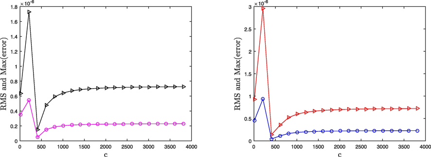
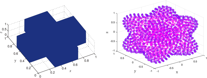
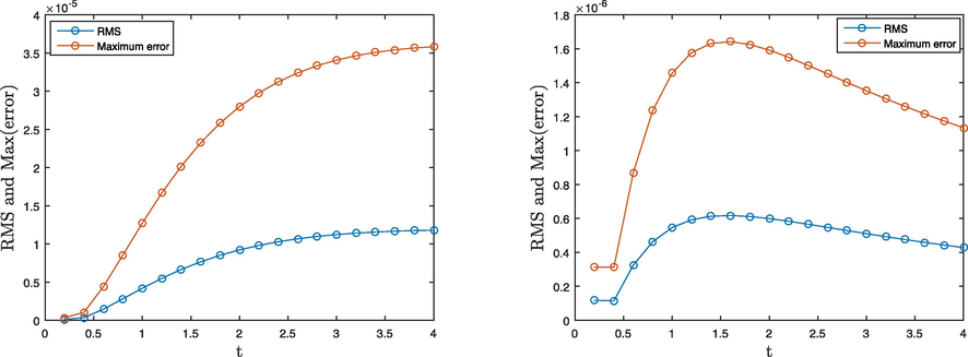
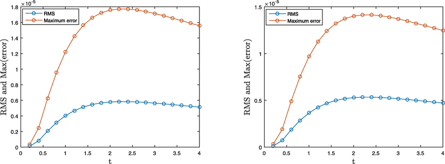
The accuracy and stability of the RBF-based meshless technique are extremely dependent on the value of the shape-parameter c, and the results will be different and unstable as the shape-parameter value changes a little. However, the accuracy and stability of the proposed technique are tested against Problem 1, as shown in Fig. 1 for (in two-term), (in three-term) and . Fig. 1 exposed that the proposed technique is accurate and stable. In the current paper, we have studied two irregular domains which are illustrated in Fig. 2. In Figs. 3 and 4, the results are shown for Problem 1 regarding the non-rectangular domains. For two-term case, we have considered the value of (for Domain-1) and (for Domain-2) whereas in case of three-term, are taken into account for both Domain-1 and Domain-2, for various time up to . These figures visualized better accuracy in both types of domains.
The exact solution for Eqs. (1), (2) with
is
Determining the accuracy of the recommended technique, results of Problem 2 are compared with the exact solution for diverse and N using for (for two-term) and (for three-term). These results are shown in Table 3. In this table, we can notice that the recommended method provides better results with few iterations and is become more accurate when iterations increase and both the error norms reached up to . In Table 4, the results are achieved using various ’s for and . Observing this table we can say that accurate results have been achieved for various time fractional orders in this problem as well.
The exact solution for Eqs. (1), (2) with
is
| Two-term | 0.1 | 2.8416e−04 | 8.8737e−05 | 2.9285e−04 | 9.2558e−05 | 2.9732e−04 | 9.5131e−05 |
| 0.05 | 7.0957e−05 | 2.2159e−05 | 7.3125e−05 | 2.3112e−05 | 7.4237e−05 | 2.3753e−05 | |
| 0.01 | 2.8334e−06 | 8.8481e−07 | 2.9195e−06 | 9.2271e−07 | 2.9633e−06 | 9.4813e−07 | |
| 0.005 | 7.0756e−07 | 2.2096e−07 | 7.2896e−07 | 2.3039e−07 | 7.3980e−07 | 2.3671e−07 | |
| 0.001 | 2.8171e−08 | 8.7973e−09 | 2.9007e−08 | 9.1677e−09 | 2.9420e−08 | 9.4132e−09 | |
| 0.0005 | 7.0184e−09 | 2.1916e−09 | 7.2236e−09 | 2.2830e−09 | 7.3231e−09 | 2.3430e−09 | |
| Three−term | 0.1 | 2.8404e−04 | 8.8701e−05 | 2.9272e−04 | 9.2515e−05 | 2.9716e−04 | 9.5082e−05 |
| 0.05 | 7.0915e−05 | 2.2146e−05 | 7.3078e−05 | 2.3097e−05 | 7.4183e−05 | 2.3736e−05 | |
| 0.01 | 2.8296e−06 | 8.8364e−07 | 2.9152e−06 | 9.2135e−07 | 2.9584e−06 | 9.4657e−07 | |
| 0.005 | 7.0624e−07 | 2.2054e−07 | 7.2744e−07 | 2.2991e−07 | 7.3807e−07 | 2.3615e−07 | |
| 0.001 | 2.8053e−08 | 8.7602e−09 | 2.8870e−08 | 9.1244e−09 | 2.9266e−08 | 9.3636e−09 | |
| 0.0005 | 6.9765e−09 | 2.1785e−09 | 7.1754e−09 | 2.2677e−09 | 7.2683e−09 | 2.3254e−09 | |
| Two-term | 0.2 | 7.3170e−07 | 2.3126e−07 | 5.3832e−07 | 1.7014e−07 | 2.9704e−07 | 9.3882e−08 |
| 0.4 | 7.3053e−07 | 2.3089e−07 | 5.3746e−07 | 1.6987e−07 | 2.9657e−07 | 9.3733e−08 | |
| 0.6 | 7.2584e−07 | 2.2940e−07 | 5.3402e−07 | 1.6878e−07 | 2.9468e−07 | 9.3134e−08 | |
| 0.8 | 7.0765e−07 | 2.2364e−07 | 5.2065e−07 | 1.6455e−07 | 2.8731e−07 | 9.0801e−08 | |
| Three−term | 0.2 | 7.3154e−07 | 2.3121e−07 | 5.3818e−07 | 1.7010e−07 | 2.9696e−07 | 9.3856e−08 |
| 0.4 | 7.2979e−07 | 2.3065e−07 | 5.3690e−07 | 1.6969e−07 | 2.9626e−07 | 9.3634e−08 | |
| 0.6 | 7.2276e−07 | 2.2843e−07 | 5.3174e−07 | 1.6805e−07 | 2.9342e−07 | 9.2735e−08 | |
| 0.8 | 6.9547e−07 | 2.1979e−07 | 5.1169e−07 | 1.6171e−07 | 2.8237e−07 | 8.9235e−08 | |
-
Problem 1, c versus error norms (left) two-term model equation, (right) three-term model equation.
-
Domain-1 (left) and Domain-2 (right).
-
Problem 1, error profile of two-term model equation (left) Domain-1 (right) Domain-2.
-
Problem 1, error profile of three-term model equation (left) Domain-1 (right) Domain-2.
| Two-term | 0.1 | 2.1364e−04 | 5.9329e−05 | 2.0995e−04 | 6.1905e−05 | 2.1083e−04 | 6.3636e−05 |
| 0.05 | 5.3362e−05 | 1.4819e−05 | 5.2441e−05 | 1.5462e−05 | 5.2659e−05 | 1.5894e−05 | |
| 0.01 | 2.1334e−06 | 5.9244e−07 | 2.0964e−06 | 6.1814e−07 | 2.1051e−06 | 6.3539e−07 | |
| 0.005 | 5.3324e−07 | 1.4808e−07 | 5.2401e−07 | 1.5451e−07 | 5.2616e−07 | 1.5881e−07 | |
| 0.001 | 2.1318e−08 | 5.9201e−09 | 2.0947e−08 | 6.1764e−09 | 2.1032e−08 | 6.3482e−09 | |
| 0.0005 | 5.3278e−09 | 1.4795e−09 | 5.2349e−09 | 1.5435e−09 | 5.2559e−09 | 1.5863e−09 | |
| Three−term | 0.1 | 2.1360e−04 | 5.9319e−05 | 2.0991e−04 | 6.1894e−05 | 2.1079e−04 | 6.3623e−05 |
| 0.05 | 5.3351e−05 | 1.4816e−05 | 5.2429e−05 | 1.5459e−05 | 5.2645e−05 | 1.5890e−05 | |
| 0.01 | 2.1326e−06 | 5.9223e−07 | 2.0956e−06 | 6.1790e−07 | 2.1042e−06 | 6.3512e−07 | |
| 0.005 | 5.3302e−07 | 1.4802e−07 | 5.2376e−07 | 1.5443e−07 | 5.2588e−07 | 1.5873e−07 | |
| 0.001 | 2.1303e−08 | 5.9159e−09 | 2.0931e−08 | 6.1715e−09 | 2.1014e−08 | 6.3426e−09 | |
| 0.0005 | 5.3232e−09 | 1.4783e−09 | 5.2297e−09 | 1.5420e−09 | 5.2502e−09 | 1.5846e−09 | |
| Two-term | 0.1 | 5.2442e−07 | 1.5463e−07 | 3.8582e−07 | 1.1376e−07 | 2.1289e−07 | 6.2772e−08 |
| 0.3 | 5.2401e−07 | 1.5451e−07 | 3.8552e−07 | 1.1367e−07 | 2.1273e−07 | 6.2724e−08 | |
| 0.7 | 5.1568e−07 | 1.5205e−07 | 3.7941e−07 | 1.1187e−07 | 2.0936e−07 | 6.1733e−08 | |
| 0.9 | 4.9040e−07 | 1.4460e−07 | 3.6082e−07 | 1.0639e−07 | 1.9911e−07 | 5.8712e−08 | |
| Three−term | 0.1 | 5.2437e−07 | 1.5461e−07 | 3.8578e−07 | 1.1375e−07 | 2.1286e−07 | 6.2763e−08 |
| 0.3 | 5.2376e−07 | 1.5443e−07 | 3.8532e−07 | 1.1361e−07 | 2.1262e−07 | 6.2691e−08 | |
| 0.7 | 5.1127e−07 | 1.5075e−07 | 3.7615e−07 | 1.1091e−07 | 2.0757e−07 | 6.1204e−08 | |
| 0.9 | 4.7334e−07 | 1.3958e−07 | 3.4827e−07 | 1.0270e−07 | 1.9219e−07 | 5.6673e−08 | |
-
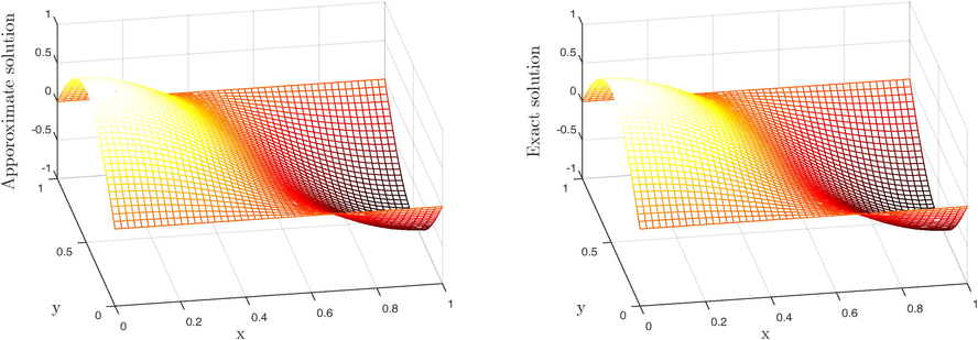
Problem 3, two-term model equation at
(left) numerical solution (right) exact solution.
-
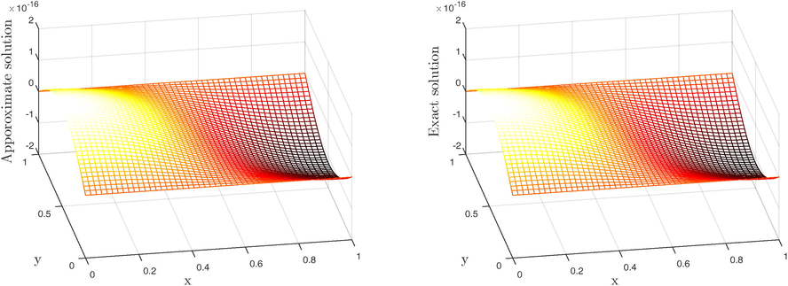
Problem 3, three-term model equation at
(left) numerical solution (right) exact solution.
4 Conclusion
In this paper, we have examined the effectiveness and applicability of the suggested local meshless technique to compute the numerical solution of time fractional Sobolev model equations. The obtained results prove that the suggested technique works amazingly in fractional PDE models. Numerical experiments show that the algorithm gives good accuracy and in light of these analyses, we suggest that the local meshless technique can be implemented to such types of fractional PDE models which appear in physical problems.
Acknowledgements
Taif university researchers supporting project number (TURSP-2020/031), Taif university, Taif, Saudi Arabia. The first author is thankful to the support of the Natural Science Foundation of Anhui Province (Project No. 1908085QA09) and the University Natural Science Research Project of Anhui Province (Project No. KJ2019A0591, KJ2020ZD008).
Funding
The authors received financial support from Taif University Researchers Supporting Project Number (TURSP-2020/031), Taif University, Taif, Saudi Arabia.
Declaration of Competing Interest
The authors declare that they have no known competing financial interests or personal relationships that could have appeared to influence the work reported in this paper.
References
- Local meshless differential quadrature collocation method for time-fractional PDEs. Discrete & Continuous Dynamical Systems-S 2018
- [Google Scholar]
- Local RBF method for multi-dimensional partial differential equations. Computers & Mathematics with Applications. 2017;74:292-324.
- [Google Scholar]
- Numerical simulation of partial differential equations via local meshless method. Symmetry. 2019;11:257.
- [Google Scholar]
- Numerical simulation of PDEs by local meshless differential quadrature collocation method. Symmetry. 2019;11(3):394.
- [Google Scholar]
- Solution of multi-term time-fractional PDE models arising in mathematical biology and physics by local meshless method. Symmetry. 2020;12(7):1195.
- [Google Scholar]
- A new analyzing technique for nonlinear time fractional Cauchy reaction-diffusion model equations. Results in Physics 2020 103462
- [Google Scholar]
- Numerical simulation of simulate an anomalous solute transport model via local meshless method. Alexandria Engineering Journal. 2020;59(4):2827-2838.
- [Google Scholar]
- Study on numerical solution of dispersive water wave phenomena by using a reliable modification of variational iteration algorithm. Mathematics and Computers in Simulation 2020
- [Google Scholar]
- Analytic approximate solutions for some nonlinear parabolic dynamical wave equations. Journal of Taibah University for Science. 2020;14(1):346-358.
- [Google Scholar]
- Modified variational iteration technique for the numerical solution of fifth order KdV type equations. J. Appl. Comput. Mech. 2020:236-242.
- [Google Scholar]
- Application of local meshless method for the solution of two term time fractional-order multi-dimensional PDE arising in heat and mass transfer. Thermal Science. 2020;24(Suppl. 1):95-105.
- [Google Scholar]
- Numerical study of integer-order hyperbolic telegraph model arising in physical and related sciences. The European Physical Journal Plus. 2020;135(9):1-14.
- [Google Scholar]
- Ain, Q.T., He, J.-H., 2019. On two-scale dimension and its applications. Thermal Science 23 (3 Part B), 1707–1712.
- Linear models of dissipation whose Q is almost frequency independent–ii. Geophysical Journal International. 1967;13(5):529-539.
- [Google Scholar]
- A tutorial review on fractal spacetime and fractional calculus. International Journal of Theoretical Physics. 2014;53(11):3698-3718.
- [Google Scholar]
- Fractal calculus and its geometrical explanation. Results in Physics. 2018;10:272-276.
- [Google Scholar]
- He, J.-H., Ain, Q.-T., 2020. New promises and future challenges of fractal calculus: from two-scale thermodynamics to fractal variational principle. Thermal Science (00), 65–65.
- Homotopy perturbation method for Fangzhu oscillator. Journal of Mathematical Chemistry. 2020;58(10):2245-2253.
- [Google Scholar]
- Periodic property of the time-fractional Kundu–Mukherjee–Naskar equation. Results in Physics. 2020;19:103345
- [Google Scholar]
- Geometrical explanation of the fractional complex transform and derivative chain rule for fractional calculus. Physics Letters A. 2012;376(4):257-259.
- [Google Scholar]
- Extension of optimal homotopy asymptotic method with use of Daftardar-Jeffery polynomials to Hirota-Satsuma coupled system of Korteweg–de Vries equations. Open Physics. 2020;18(1):916-924.
- [Google Scholar]
- Analysing time-fractional exotic options via efficient local meshless method. Results in Physics. 2020;103385
- [Google Scholar]
- Khan, M.N., Siraj-ul-Islam, Hussain, I., Ahmad, I., Ahmad, H., 2020. A local meshless method for the numerical solution of space-dependent inverse heat problems. Mathematical Methods in the Applied Sciences.
- He–Laplace method for nonlinear vibration systems and nonlinear wave equations. Journal of Low Frequency Noise, Vibration and Active Control. 2019;38(3–4):1060-1074.
- [Google Scholar]
- An extension of optimal auxiliary function method to fractional order high dimensional equations. Alexandria Engineering Journal. 2021;60(5):4809-4818.
- [Google Scholar]
- Differential Quadrature and Its Application in Engineering. London: Springer-Verlag; 2000.
- Numerical simulation of three-dimensional fractional-order convection-diffusion PDEs by a local meshless method. Thermal Science 2020:210.
- [Google Scholar]
- The method of fundamental solutions for steady-state groundwater flow problems. Journal of the Chinese Institute of Engineers. 2016;39(2):236-242.
- [Google Scholar]
- Optimality of the boundary Knot method for numerical solutions of 2D Helmholtz-type equations. Wuhan University Journal of Natural Sciences. 2019;24(4):314-320.
- [Google Scholar]
- Formation of intermetallic phases in ion implantation. Journal of Mathematics. 2020;2020
- [Google Scholar]
- Gaussian radial basis functions method for linear and nonlinear convection–diffusion models in physical phenomena. Open Physics. 2021;19(1):69-76.
- [Google Scholar]
Appendix A
Supplementary data
Supplementary data associated with this article can be found, in the online version, at https://doi.org/10.1016/j.jksus.2021.101604.
Supplementary data
The following are the Supplementary data to this article:


