

Translate this page into:
Magnetic anomaly interpretation for a 2D fault-like geologic structures utilizing the global particle swarm method
⁎Corresponding author. khalid_sa_essa@yahoo.com (Khalid S. Essa)
-
Received: ,
Accepted: ,
This article was originally published by Elsevier and was migrated to Scientific Scholar after the change of Publisher.
Peer review under responsibility of King Saud University.
Abstract
We establish a method to interpret the magnetic anomaly due to 2D fault structures, with an evaluation of first moving average residual anomalies utilizing filters of increasing window lengths. After that, the buried fault parameters are estimated using the global particle swarm method. The goodness of fit among the observed and the calculated models is expressed as the root mean squared (RMS) error. The importance of studying and delineating the fault parameters, which include the amplitude factor, the depth to the upper edge, the depth to the lower edge, the fault dip angle, and the position of the origin of the fault, is: (i) solving many problem-related engineering and environmental applications, (ii) describing the accompanying mineralized zones with faults, (iii) describing geological deformation events, (iv) monitoring the subsurface shear zones, (v) defining the environmental effects of the faults before organizing any investments, and (vi) imaging subsurface faults for different scientific studies.
Finally, we show the method applied to two theoretical models including the influence of the regional background and the multi-fault effect and to real field examples from Australia and Turkey. Available geologic and geophysical information corroborates our interpretations.
Keywords
Global particle swarm
Moving average
Fault
Depth

1 Introduction
The magnetic method uses the magnetization contrasts between different lithologies to examine environmental or geologic subsurface problems of various kinds. These problems include subsurface elements and mineral and ore detection (Al-Garni, 2010; Dar and Bukhari, 2020; Mehanee et al., 2021; Ben et al., 2022a; Saada et al., 2022; Ekwok et al., 2023), hydrocarbon exploration (Osinowo and Taiwo, 2020), archaeological investigation (Essa and Abo-Ezz, 2021), geotechnical engineering (Igwe and Umbugadu, 2020), cave discovery (Orfanos and Apostolopoulos, 2012) and geothermal exploration (Abraham and Alile, 2019). Inversion of magnetic data for arbitrarily complex structure is an ill-posed and non-unique problem (Utsugi, 2019). Interpretation for simple geometric shapes reduces the complexity and offers usable best-fit solutions (Abo-Ezz and Essa, 2016; Essa and Elhussein, 2019; Biswas and Rao, 2021; Ben et al., 2022b).
Graphical and numerical methods have long been used to appraise simple subsurface geometric-model parameters (Gay, 1963; Abdelrahman et al., 2009; Biswas et al., 2017). Global optimization algorithms have been successfully applied to full complete interpretation (Biswas and Acharya, 2016; Ekinci et al., 2019; Di Maio et al., 2020; Essa, 2021; Essa et al., 2021; Singh and Biswas, 2021; Biswas et al., 2022; Ai et al., 2023).
In this study we present an extended application of the particle swarm method to elucidate the magnetic residual anomaly of 2D fault-like geologic structures. A residual magnetic anomaly is computed using a first moving average to estimate a first-order regional from the observed magnetic anomaly. The proposed method was verified on two theoretical examples. The first example demonstrates the influence of the linear regional field and the second example shows the detection of subsurface multi-faults. The appraised fault parameters (K, z1, z2, θ, β, and c – see Fig. 1) show that the proposed method is firm. After that, the suggested method was applied on two real datasets from Australia and Turkey to obtain the subsurface fault parameters. Finally, the results from the examples studied show that the proposed method can tolerate noise and regional background in the observed field and give a good insight into subsurface faults.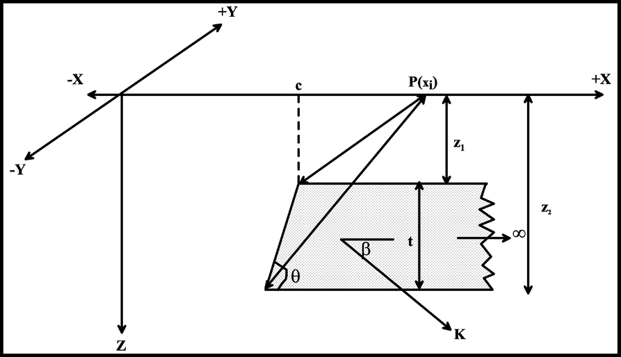
Sketch diagram for a two-dimensional (2D) fault-like geologic structure and its parameters.
2 Particle swarm method
The particle swarm optimization is carefully distinguished and has been used to address a variety of geophysical problems. The development of the method was fully described in the published literature (Singh and Biswas, 2016; Essa and Munschy, 2019; Essa, 2021), and we do not repeat it here. Instead, we accentuation on its considerable profits in vanquishing the ill-posedness and non-uniqueness of magnetic data inversion. Furthermore, it is firm, vigorous, and effective in attaining an optimal global solution. The power of the technique is typically seen in the theoretical and field models presented below.
3 Forward modelling
For a 2D fault model, the magnetic anomaly (T) at an observation point (P(xj)) along a profile (Fig. 1) is given by (e.g., Murthy et al., 2001; Aydin, 2008):
4 First moving average method
The total magnetic field anomaly can be decomposed as a residual and a respectively linear regional field, which are related to shallow and deep geologic structures, is:
Griffin (1949) explained that the first moving average regional is:
The particle swarm optimization method is utilized to the residual (calculated above) to obtain the 2D fault parameters (K, z1, z2, θ, β, and c).
Finally, the optimum magnetic anomaly fit is reached by seeking the minimum RMS misfit (λ), which is defined as:
where N is the number of measured points,
is the observed magnetic anomaly and
is the calculated anomaly at the point xj. Fig. 2 displays the flow diagram for the proposed method.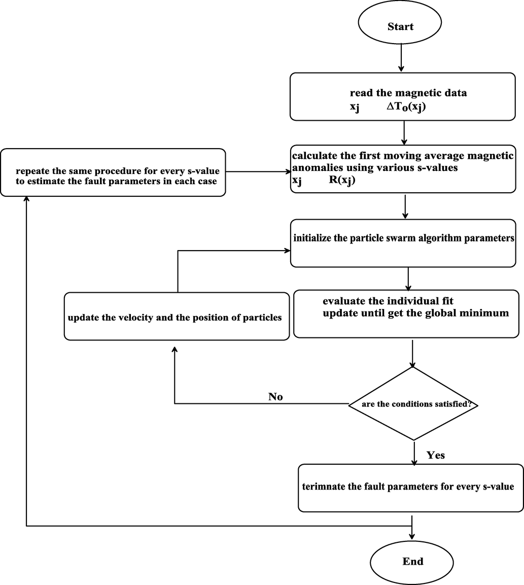
Flow-chart for the suggested approach.
5 Theoretical models
We investigated the uncertainties and stability of the suggested technique for assessing the 2D fault model parameters (K, z1, z2, θ, β, and c) by studying the following two theoretical examples, which revealed the impact of imposed linear regional background and multi-faults effects exemplified by a horst.
5.1 Model 1: Impact of linear regional field
This composite model uses the expected magnetic anomaly (ΔTo) for the 2D fault described by Equation (1) with the parameters: K = 400 nT, z1 = 4 km, z2 = 7 km, θ = 35°, β = 30°, c = 50 km, and profile length = 100 km and the influence of some unknown deep-structure (regional anomaly) representing by a first-order polynomial
(Fig. 3a).
(a) Composite theoretical magnetic anomaly (Model 1). (b) First moving average residual magnetic anomalies for the anomaly in Fig. 3a. (c) Noisy magnetic anomaly. (d) First moving average residual magnetic anomalies for anomaly in Fig. 3c. (e) Geologic sketch of the 2D fault model. (f) Observed and evaluated anomalies misfits in all cases.
We have applied the moving average method to estimate the first moving average residual anomalies by implementing equation (4) applying several window lengths (s = 3, 5, 7, 9, and 11 km) (Fig. 3b). Next, the particle swarm was used to gauge the 2D fault parameters (K, z1, z2, θ, β, and c) (Table 1). In Table 1, the ranges used for all parameters are presented and the results of the estimated fault parameters are: K = 399.08 ± 0.65 nT, z1 = 3.99 ± 0.01 km, z2 = 6.99 ± 0.01 km, θ = 34.99 ± 0.02°, β = 29.99 ± 0.02°, and c = 49.99 ± 0.02 km. The errors in each parameter are vanishingly small and the RMS misfit among the original and the estimated anomalies is 0.22 nT (Fig. 3f). For a noise-free model, this is gratifying but unsurprising.
Parameters
Used ranges
Applying the particle swarm method for the first moving average magnetic data
with a 0% noise level
s = 3 km
s = 5 km
s = 7 km
s = 9 km
s = 11 km
μ
δ (%)
λ (nT)
K (nT)
100–1000
398.23
398.67
399.14
399.50
399.86
399.08 ± 0.65
0.23
0.22
z1 (km)
1–20
3.99
3.99
4.00
3.99
4.00
3.99 ± 0.01
0.15
z2 (km)
1–20
6.98
6.98
7.00
7.01
6.99
6.99 ± 0.01
0.11
θ (o)
10–80
34.96
34.99
34.99
34.99
35.00
34.99 ± 0.02
0.04
β (o)
10–80
29.97
29.99
30.01
30.00
30.00
29.99 ± 0.02
0.02
c (km)
10–100
49.98
49.98
49.98
50.01
50.01
49.99 ± 0.02
0.02
with a 10% noise level
K (nT)
100–1000
382.95
383.13
387.47
389.69
390.24
386.70 ± 3.50
3.33
22.01
z1 (km)
1–20
3.74
3.80
3.84
3.87
3.92
3.83 ± 0.07
4.15
z2 (km)
1–20
6.71
6.75
6.77
6.81
6.85
6.78 ± 0.05
3.17
θ (o)
10–80
32.98
33.36
33.61
34.12
34.38
33.69 ± 0.57
3.74
β (o)
10–80
27.63
28.02
28.14
28.56
29.06
28.28 ± 0.55
5.73
c (km)
10–100
47.56
47.88
49.15
49.30
49.67
48.71 ± 0.93
2.58
This method’s performance was examined after inserting 10% random noise on the above composite magnetic anomaly (Fig. 3c) applying the next form:
Application of the moving average method with the same window lengths yielded noisy residual magnetic anomalies (Fig. 3d). The global particle swarm optimization gave estimated buried fault structure parameters (Table 1). Table 1 reveals each parameter result as follows: K = 386.70 ± 3.50 nT, z1 = 3.83 ± 0.07 km, z2 = 6.78 ± 0.05 km, θ = 33.69 ± 0.57°, β = 28.28 ± 0.55°, and c = 48.71 ± 0.93 km, with 3.33%, 4.15%, 3.17%, 3.74%, 5.73%, and 2.58%, respectively. The misfit (λ = 22.01 nT) amongst the observed anomaly and the assessed magnetic anomalies is revealed in Fig. 3f.
The results for 0% and 10% noise level imposed on the composite magnetic anomaly reveals the suggested method was capable to cope with the regional background and noise and created valid results.
5.2 Model 2: Multi-fault consisting of a horst
We examined a 100 km composite magnetic profile due to multi-fault structures consisting of a horst block with the following parameters: K1 = 300 nT, z11 = 3 km, z21 = 10 km, θ1 = 120°, β1 = 20°, and c1 = 53 km for body 1 and K2 = 200 nT, z12 = 5 km, z22 = 10 km, θ2 = 135°, β2 = 20°, and c2 = 47 km for body 2 along 100 km profile (Fig. 4a and 4e).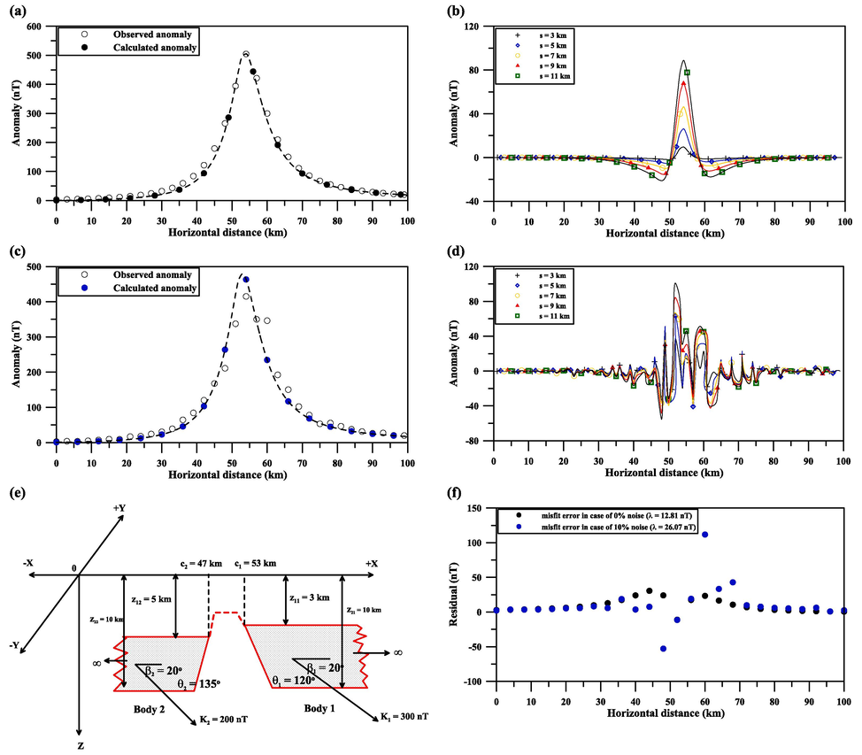
Composite theoretical magnetic anomaly (Model 2). (b) First moving average residual magnetic anomalies for anomaly in Fig. 4a. (c) Noisy magnetic anomaly. (d) First moving average residual magnetic anomalies for the anomaly in Fig. 4c. (e) 2D fault sketch. (f) Observed and evaluated magnetic anomalies misfits in all cases.
The first moving average method was employed to the magnetic anomaly exploiting several s-values (s = 3, 5, 7, 9, and 11 km) (Fig. 4b); subsequent the particle swarm method was claimed in order to assess the subsurface faults structures parameters (Table 2). Table 2 indicates the outcomes for the two fault structures, which consist of a horst block, which are: K1 = 290.56 ± 3.96 nT, z11 = 2.93 ± 0.02 km, z21 = 10.00 ± 0.05 km, θ1 = 118.18 ± 0.84°, β1 = 19.46 ± 0.47°, and c1 = 52.59 ± 0.35 km, and the error of K1, z11, z21, θ1, β1, and c1 are: 3.15%, 2.33%, 0%, 1.52%, 2.72%, and 0.77%, respectively, while the calculated parameters of the second model (Body 2; Fig. 4e) are: K2 = 195.17 ± 2.031 nT, z12 = 4.78 ± 0.15 km, z22 = 8.92 ± 0.50 km, θ2 = 134.04 ± 3.06°, β2 = 18.97 ± 0.73°, and c2 = 46.22 ± 0.62 km, and the error of K2, z12, z22, θ2, β2, and c2 are: 2.41%, 4.48%, 10.76%, 0.71%, 5.16%, and 1.66%, correspondingly, and the RMS misfit (λ-value) is 12.81 nT.
Model
Parameters
Used ranges
Applying the particle swarm method for the first moving average magnetic data
with a 0% noise level
s = 3 km
s = 5 km
s = 7 km
s = 9 km
s = 11 km
μ
δ (%)
λ (nT)
Body1
K (nT)
100–500
285.13
288.10
291.32
293.27
294.96
290.56 ± 3.96
3.15
12.81
z1 (km)
1–20
2.91
2.91
2.95
2.93
2.95
2.93 ± 0.02
2.33
z2 (km)
1–20
9.84
9.87
9.92
9.93
9.96
10.00 ± 0.05
0
θ (o)
10–170
117.11
117.64
118.14
119.02
119.00
118.18 ± 0.84
1.52
β (o)
10–80
18.81
19.19
19.50
19.85
19.93
19.46 ± 0.47
2.72
c (km)
10–100
52.05
52.48
52.66
52.84
52.94
52.59 ± 0.35
0.77
Body2
K (nT)
100–500
192.09
194.26
195.72
196.90
196.88
195.17 ± 2.03
2.41
z1 (km)
1–20
4.58
4.70
4.76
4.92
4.92
4.78 ± 0.15
4.48
z2 (km)
1–20
8.23
8.68
8.94
9.23
9.54
8.92 ± 0.50
10.76
θ (o)
10–170
129.44
132.31
136.00
136.05
136.38
134.04 ± 3.06
0.71
β (o)
10–80
18.06
18.42
19.02
19.54
19.80
18.97 ± 0.73
5.16
c (km)
10–100
45.33
45.94
46.28
46.61
46.94
46.22 ± 0.62
1.66
with a 10% noise level
Body1
K (nT)
100–500
271.24
276.76
283.81
285.25
293.59
282.13 ± 8.53
5.96
26.07
z1 (km)
1–20
2.82
2.86
2.90
3.01
2.97
2.91 ± 0.08
2.93
z2 (km)
1–20
8.75
9.10
10.12
9.91
9.93
9.56 ± 0.60
4.38
θ (o)
10–170
114.36
116.71
118.25
121.48
123.81
118.92 ± 3.76
0.90
β (o)
10–80
18.19
20.03
19.86
20.57
21.14
19.96 ± 1.11
0.21
c (km)
10–100
50.48
51.05
51.74
52.60
53.25
51.82 ± 1.12
2.22
Body2
K (nT)
100–500
185.03
188.17
193.44
199.00
204.13
193.95 ± 7.78
3.02
z1 (km)
1–20
4.41
4.74
4.92
5.13
5.20
4.88 ± 0.32
2.40
z2 (km)
1–20
8.15
8.49
9.26
9.74
10.04
9.14 ± 0.80
8.64
θ (o)
10–170
130.36
132.06
133.57
134.61
134.85
133.09 ± 1.88
1.41
β (o)
10–80
17.47
18.11
18.85
18.92
19.53
18.58 ± 0.80
7.12
c (km)
10–100
46.22
47.23
47.62
47.85
47.85
47.35 ± 0.68
0.75
We then imposed a 10% random error on the anomaly (Fig. 4c) using the previous (Eq. (6). The first moving average residual magnetic anomalies were calculated using the same s-values as before (Fig. 4d), and the fault parameters estimated via the global particle swarm method (Table 2). As shown in Table 2, the predicated parameters of the first model (Body 1; Fig. 4e) are: K1 = 282.13 ± 8.53 nT, z11 = 2.91 ± 0.08 km, z21 = 9.56 ± 0.60 km, θ1 = 118.92 ± 3.76°, β1 = 19.96 ± 111°, and c1 = 51.82 ± 1.12 km, and the errors in K1, z11, z21, θ1, β1, and c1 are: 5.96%, 2.93%, 4.38%, 0.90%, 0.21%, and 2.22%, respectively, while the estimated parameters of the second model (Body 2; Fig. 4e) are: K2 = 193.95 ± 7.78 nT, z12 = 4.88 ± 0.32 km, z22 = 9.14 ± 0.80 km, θ2 = 133.09 ± 1.88°, β2 = 18.58 ± 0.80°, and c2 = 47.35 ± 0.68 km, and the error of K2, z12, z22, θ2, β2, and c2 are: 3.02%, 2.40%, 8.64%, 1.41%, 7.12%, and 0.75%, correspondingly, with an RMS misfit of 26.07 nT.
The misfit amongst the original anomaly and the calculated anomaly (Fig. 4a and Fig. 4c) is shown in Fig. 4f.
In summary, the particle swarm method has been employed on two theoretical models, which represent the effect of a linear regional background and noise (Model 1), and the effect of multi-faults (Model 2). A respectable match of the observed to the calculated model parameters has been found and the errors in all assessed parameters do not increase more than 10%.
6 Real data examples
To inspect the practical applicability of the proposed method, two real data sets were collected from the available published literature from Australia and Turkey. The particle swarm method was used to invert the observed magnetic field values to achieve the optimum fit of the fault parameters (K, z1, z2, θ, β, and c), which were then compared with current geologic information and any additional geophysical outcomes.
6.1 The Perth basin field example, Australia
The Perth Basin is placed at the western part of Australia and is elongated north-to-south. It is effectively the southern part of the Carnarvon Basin and covers an area of about 100,000 km2. It is considered as an important basin for hydrocarbon exploration in Australia and includes more than twenty commercial oil and gas fields. The Perth Basin is a huge rift structure, which formed during intra-continental rifting and developed through eventual division of India from Australia. This basin is separated to fifteen sub-basins, which record a big sedimentary fill ranging from Permian to Recent age (Harris, 1994; Olierook et al., 2015) (Fig. 5a).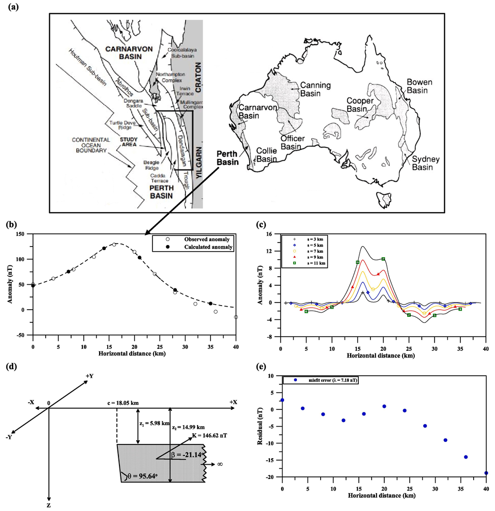
(a) Location and geologic map of the Perth Basin, Western Australia (after Mory and Iasky, 1996). (b) Observed and calculated magnetic anomalies for the Perth Basin field example, Australia. (c) First moving average residual magnetic anomalies for the anomaly in Fig. 5b. (d) Geologic model of the evaluated 2D fault. (e) Observed and evaluated magnetic anomalies misfit.
The observed magnetic anomaly owing to a fault-like geologic structure was collected at the Western border of the Perth basin, Australia (Qureshi and Nalaye 1978). The profile length of 40 km was digitized at 1 km intervals (Fig. 5b). This digitized anomaly was used to gauge the parameters K, z1, z2, θ, β, and c using the proposed method for available first moving average residual magnetic anomalies (Fig. 5c) using s = 3, 5, 7, 9, and 11 km (Table 3). Table 3 demonstrates the extents and results of the fault model parameters as follows: K = 146.62 ± 1.04 nT, z1 = 5.98 ± 0.26 km, z2 = 14.99 ± 0.35 km, θ = 95.64 ± 0.29°, β = -21.14 ± 1.92°, and c = 18.05 ± 0.42 km. The misfit (RMS value, λ = 7.18 nT) of the original anomaly and the predicated magnetic anomalies is given in profile in Fig. 5e.
Parameters
Used ranges
Applying the particle swarm method for the first moving average magnetic data
s = 3 km
s = 5 km
s = 7 km
s = 9 km
s = 11 km
μ
λ (nT)
K (nT)
50–500
145.19
146.03
146.72
147.34
147.80
146.62 ± 1.04
7.18
z1 (km)
1–20
5.65
5.87
5.93
6.12
6.34
5.98 ± 0.26
z2 (km)
1–20
14.58
14.76
14.98
15.17
15.48
14.99 ± 0.35
θ (o)
10–170
95.27
95.68
95.42
95.91
95.91
95.64 ± 0.29
β (o)
−80-+80
−18.84
−19.59
−21.35
–22.48
–23.43
−21.14 ± 1.92
c (km)
5–40
17.41
17.90
18.24
18.53
18.17
18.05 ± 0.42
The estimated fault parameters by the application of the global particle swarm convolved with the first moving average have a respectable agreement with the results achieved from borehole information (Qureshi and Nalaye (1978); z1 = 5.80 to 6.85 km, z2 = 15.55 to 17 km, θ = 30°) and additional interpretation methods, for example; Rao and Babu (1983) estimated the parameters as follows: z1 = 6.26 km, z2 = 15.45 km, θ = 40°. Tlas and Asfahani (2011) calculated the parameters K = 200.56 nT, z1 = 7.22 km, z2 = 13.72 km, θ = 35.56°. Di Maio et al. (2020) interpreted the fault parameters as follows: K = 169.40 nT, z1 = 8.50 km, z2 = 12 km, θ = 35.86°. In more detail, the previous inversion methods used the observed magnetic anomaly as a residual anomaly, with no attempt to remove a regional, which is not clear in the respective papers.
6.2 The Şereflikoçhisar-Aksaray fault field example, Turkey
The city of Aksaray is situated in the southwest of the central part of Anatolia between the Sakarya Region and Pontides (Eurasian Plate) in the north and the Anatolide-Tauride Platform in the south. The area is surrounded by young sediments consisting of tertiary units and surrounded by massive metamorphic rocks, comprised of mica schists, graphite schists, phyllites quartzites and marbles. Also, a granitoid intrusion is found in the eastern part of the Şereflikoçhisar-Aksaray fault and Cappadocian volcanic rocks occasioned from tectonic activities due to the subduction of the Neo-Tethys Ocean. (Aydemir and Ates, 2006; Bilim et al., 2015) (Fig. 6a).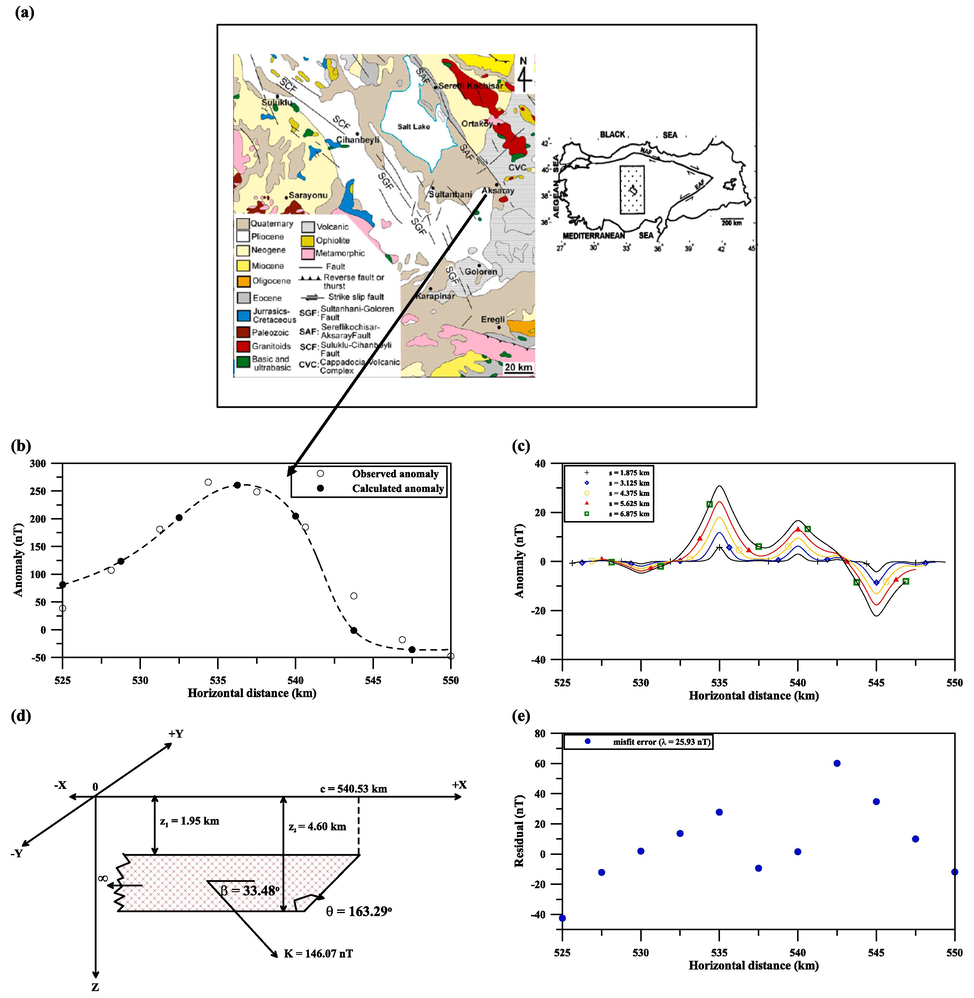
(a) Location and geologic map of the Şereflikoçhisar-Aksaray fault field example, Turkey (after Bilim et al., 2015). (b) Observed and the calculated magnetic anomalies for the Aksaray fault field example, Turkey. (c) First moving average residual magnetic anomalies for the anomaly in Fig. 6b. (d) Geologic model of the buried 2D fault. (e) Observed and calculated anomalies misfit.
The magnetic anomaly profile for the Aksaray fault, Turkey (Aydemir and Ates, 2006; Fig. 6) with a length of 25 km and digitized at an interim of 0.625 km (Fig. 6b) was employed. A complete interpretation of this magnetic anomaly was done by applying the same procedure as above. The first moving average residual magnetic anomalies were achieved for numerous window lengths (s = 1.875, 3.125, 4.375, 5.625, and 6.875 km) (Fig. 6c). The particle swarm method was employed to these anomalies to evaluate the fault parameters (Table 4). The results in Table 4 are: K = 146.07 ± 1.38 nT, z1 = 1.95 ± 0.07 km, z2 = 4.60 ± 0.15 km, θ = 163.29 ± 0.98°, β = 33.48 ± 0.49°, and c = 540.53 ± 2.83 km. As well, the misfit (RMS value λ = 25.93 nT) among the observed anomaly and the estimated magnetic anomalies is depicted in Fig. 6e. Lastly, the fault model parameters estimated by the proposed method show good agreement with published values, especially the depths to the top and bottom, from Aydemir and Ates (2006) (z1 = 1.92 km and z2 = 4.61 km).
Parameters
Used ranges
Applying the particle swarm method for the first moving average magnetic data
s = 1.875 km
s = 3.125 km
s = 4.375 km
s = 5.625 km
s = 6.875 km
μ
λ (nT)
K (nT)
50–500
144.14
145.35
147.72
146.28
146.84
146.07 ± 1.38
25.93
z1 (km)
1–20
1.86
1.91
1.95
2.04
1.98
1.95 ± 0.07
z2 (km)
1–20
4.53
4.46
4.51
4.67
4.83
4.60 ± 0.15
θ (o)
10–170
162.09
162.67
163.10
164.15
164.42
163.29 ± 0.98
β (o)
5–80
32.96
33.08
33.42
33.83
34.11
33.48 ± 0.49
c (km)
525–550
536.18
539.21
541.83
542.34
543.08
540.53 ± 2.83
7 Conclusions
The application of the particle swarm method for interpreting the first moving average residual magnetic anomalies, which is produced from the observed magnetic anomaly using several window lengths, is likely to be useful in geophysical exploration, including hydrocarbon, mineral and ore exploration because it offers several benefits, namely: (1) it removes the effect of deep structures (regional background response), (2) it eliminates the effect of neighbouring structures and noise response, (3) it infers the fault model parameters with a good accuracy, and (4) the method is automatic. The accuracy and pertinence of the proposed method were verified by examining two appropriate theoretical models and two real data sets from Australia and Turkey. From results demonstrate that, the proposed method is robust and stable. This method can be extended to more complicated cases, which we propose to do in a future study.
Acknowledgments
Authors would like to thank Prof. Omar Al-Dossary, Editor-in-Chief, and the two capable reviewers for their keen interest, valuable comments on the manuscript, and improvements to this work.
Declaration of competing interest
The authors declare that they have no known competing financial interests or personal relationships that could have appeared to influence the work reported in this paper.
References
- A least-squares standard deviation method to interpret magnetic anomalies due to thin dikes. Near. Surf. Geophys.. 2009;7:41-46.
- [Google Scholar]
- A least-squares minimization approach for model parameters estimate by using a new magnetic anomaly formula. Pure Appl. Geophys.. 2016;173:1265-1278.
- [Google Scholar]
- Modelling subsurface geologic structures at the Ikogosi geothermal field, southwestern Nigeria, using gravity, magnetics and seismic interferometry techniques. J. Geophys. Eng.. 2019;16:729-741.
- [Google Scholar]
- Inversion of geomagnetic anomalies caused by ore masses using Hunger Games Search algorithm. Earth Space Sci. 2023;10:e2023EA003002
- [Google Scholar]
- Magnetic survey for delineating subsurface structures and estimating magnetic sources depth, Wadi Fatima, KSA. J. King Saud Univ. Sci.. 2010;22:87-96.
- [Google Scholar]
- Interpretation of Suluklu-Cihanbeyli-Goloren Magnetic Anomaly, Central Anatolia, Turkey: An integration of geophysical data. Phys. Earth Planet. Inter.. 2006;159:167-182.
- [Google Scholar]
- Estimation of the location and depth parameters of 2D magnetic sources using analytical signals. J. Geophys. Eng.. 2008;5:281-289.
- [Google Scholar]
- A novel method for estimating model parameters from geophysical anomalies of structural faults using the Manta-Ray foraging optimization. Front. Earth Sci.. 2022;10:870299
- [Google Scholar]
- Interpretation of magnetic anomalies by simple geometrical structures using the Manta-Ray foraging optimization. Front. Earth Sci.. 2022;10:849079
- [Google Scholar]
- Determination of block rotations and the Curie Point Depths of magnetic sources along the NW–SE-trending Sülüklü–Cihanbeyli-Gölören and Şereflikoçhisar-Aksaray Fault Zones, Central Anatolia, Turkey. Geodin. Acta. 2015;27:202-2012.
- [Google Scholar]
- A very fast simulated annealing method for inversion of magnetic anomaly over semi-infinite vertical rod-type structure. Model. Earth Syst. Environ.. 2016;2:198.
- [Google Scholar]
- Global nonlinear optimization for the interpretation of source parameters from total gradient of gravity and magnetic anomalies caused by thin dyke. Ann. Geophys.. 2017;60:G0218.
- [Google Scholar]
- Interpretation of magnetic anomalies over 2D fault and sheet-type mineralized structures using very fast simulated annealing global optimization: An understanding of uncertainty and geological implications. Lithosphere. 2021;2021:2964057.
- [Google Scholar]
- Inverse modeling and uncertainty assessment of magnetic data from 2D thick dipping dyke and application for mineral exploration. J. Appl. Geophys.. 2022;207:104848
- [Google Scholar]
- Characteristics of magnetic anomalies and subsurface structure constraints of Balapur fault in Kashmir basin, NW Himalaya. Phys. Earth Planet. Inter.. 2020;309:106599
- [Google Scholar]
- Modeling of magnetic anomalies generated by simple geological structures through Genetic-Price inversion algorithm. Phys. Earth Planet. Inter.. 2020;305:106520
- [Google Scholar]
- Parameter estimations from gravity and magnetic anomalies due to deep-seated faults: differential evolution versus particle swarm optimisation. Turk. J. Earth Sci.. 2019;28:860-881.
- [Google Scholar]
- Particle Swarm Optimization (PSO) of high-quality magnetic data of the Obudu basement complex, Nigeria. Minerals. 2023;13:1209.
- [Google Scholar]
- Evaluation of the parameters of fault-like geologic structure from the gravity anomalies applying the particle swarm. Environ. Earth Sci.. 2021;80:489.
- [Google Scholar]
- Potential field data interpretation to detect the parameters of buried geometries by applying a nonlinear least-squares approach. Acta Geod. Geophys.. 2021;56:387-406.
- [Google Scholar]
- Magnetic interpretation utilizing a new inverse algorithm for assessing the parameters of buried inclined dike-like geologic structure. Acta Geophys.. 2019;67:533-544.
- [Google Scholar]
- Fault parameters assessment from the gravity data profiles using the global particle swarm optimization. J. Pet. Sci. Eng.. 2021;207:109129
- [Google Scholar]
- Gravity data interpretation using the particle swarm optimization method with application to mineral exploration. J. Earth Syst. Sci.. 2019;128:123.
- [Google Scholar]
- Standard curves for interpretation of magnetic anomalies over long tabular bodies. Geophysics. 1963;28:161-200.
- [Google Scholar]
- Structural and tectonic synthesis for the Perth Basin, Western Australia. J. Pet. Geol.. 1994;17:129-156.
- [Google Scholar]
- Characterization of structural failures founded on soils in Panyam and some parts of Mangu, Central Nigeria. Geoenviron. Disasters. 2020;7:7.
- [Google Scholar]
- Magnetic data interpretation using a new R-parameter imaging method with application to mineral exploration. Nat. Resour. Res.. 2021;30:77-95.
- [Google Scholar]
- Mory AJ, Iasky RP (1996) Stratigraphy and structure of the onshore northern Perth Basin, Western Australia. Geological Survey of Western Australia, Report 46.
- Automatic inversion of magnetic anomalies of faults. Comput. Geosci.. 2001;27:315-325.
- [Google Scholar]
- 3D structural and stratigraphic model of the Perth Basin, Western Australia: Implications for subbasin evolution. Aust. J. Earth Sci.. 2015;62:447-467.
- [Google Scholar]
- Analysis of different geophysical methods in the detection of an underground opening at a controlled test site. J. Balkan Geophys. Soc.. 2012;15:7-18.
- [Google Scholar]
- Analysis of high-resolution aeromagnetic (HRAM) data of Lower Benue Trough, Southeastern Nigeria, for hydrocarbon potential evaluation. NRIAG J. Astron. Geophys.. 2020;9:350-361.
- [Google Scholar]
- A method for the direct interpretation of magnetic anomalies caused by two-dimensional vertical faults. Geophysics. 1978;43:179-188.
- [Google Scholar]
- Standard curves for the interpretation of magnetic anomalies over vertical faults. Geophys. Res. Bull.. 1983;21:71-89.
- [Google Scholar]
- Understanding the structural framework controlling the sedimentary basins from the integration of gravity and magnetic data: A case study from the east of the Qattara Depression area, Egypt. J. King Saud Univ. Sci.. 2022;34:101808
- [Google Scholar]
- Application of global particle swarm optimization for inversion of residual gravity anomalies over geological bodies with idealized geometries. Nat. Resour. Res.. 2016;25:297-314.
- [Google Scholar]
- Global particle swarm optimization technique in the interpretation of residual magnetic anomalies due to simple geo-bodies with idealized structure. Basics Comput. Geophys.. 2021;1:13-32.
- [Google Scholar]
- A new best-estimate methodology for determining magnetic parameters related to field anomalies produced by buried thin dikes and horizontal cylinder-like structures. Pure Appl. Geophys.. 2011;168:861-870.
- [Google Scholar]
- 3-D inversion of magnetic data based on the L1–L2 norm regularization. Earth Planets Space. 2019;71:73.
- [Google Scholar]


