Landscape geometry-based percolation of traffic in several populous cities around the world

1 Introduction

Traffic congestion has become a critical problem faced by populous cities around the world (Abdullah and Khairurrijal, 2007; Wen, 2008; Wen et al., 2019). The increasing travel demand along with growing economic potential and population densities will burden the road infrastructure (Çolak et al., 2016). An increase in the total of vehicles that by far exceeds the expansion of roads has resulted in high congestion level on many road lines, causing inconvenience in various aspects, such as time lost, fuel inefficiency, air and sound pollution, etc. (Abdullah and Khairurrijal, 2007; Wen, 2008). Traffic transition from a free flow to a seriously congested state occurs on a daily basis in populous cities and deteriorates the system’s efficiency (Wang et al., 2015). High concentrations of CO are identified as occurring in areas having heavy traffic congestion, and up to 95% of these emissions are convinced to originate from automobile exhaust (Miller, 2011). Based on the 2005 Urban Mobility Report, completed by the Texas Transportation Institute (TTI) after examining 83 metropolitan areas in the US: (a) The time wasted due to traffic jams annually increased to 62 h per peak period traveler in 2000, from 16 h in 1982. (b) The percentage of the congested road system rose to 59% in 2003, compared to 34% in 1982. (c) The number of congestion hours rose to 7.1 h in 2003, compared to 4.5 h in 1982. (d) In the United States, traffic congestion cost $63 billion in 2003 and 3.7 billion hours lost each year (Toth, 2007). In the TomTom 2013 report, it was reported that in cities like Rio de Janeiro, Mexico City, Moscow, Istanbul and Beijing, people spend on average of 475% extra time traveling due to traffic. The loss of time, money and energy, pollution, infrastructure damage, and CO₂ emissions are borne by city residents and travelers (Çolak et al., 2016). Nowadays, congestion that continues to increase and worsen becomes one of the crucial issues that challenge most modern societies, especially planners and policymakers (Barthelemy, 2016; DeWeerdt, 2016).

In some cases, to some extent, congestion can be accepted by residents, as long as the urban system can provide high overall accessibility. More broadly, congestion can be used as a sign of the presence of agglomeration, economic growth, and city dynamics (ECMT, 2007). Statistical analysis on 30 years of data to evaluate the impacts of regional traffic congestion in 89 metropolitan areas across the US concluded that traffic congestion does not slow down economy, productivity, or job growth. Instead, a city without jamming would mean something is wrong. There would be less stimulus for infill development, living in an efficient place, walking, cycling, innovations in urban freight, etc. (Lutenegger, 2018). The congestion is a sign of vibrant city. No one wants to live in or visit a city without congestion (Hume, 2017). Congestion may lead to concentrations of certain industries (high tech and professional services) that are not much impacted by congestion (Lutenegger, 2018). Traffic congestion can promote economic growth. However, at one point, it indeed becomes a drag on the economy (Hume, 2017). Therefore, the essential thing in a policy is not to eradicate congestion, but how to manage it to avoid excessive congestion (ECMT, 2007). This context is what encourages researchers to understand traffic in various aspects, from vehicle movement, network topology to urban planning.

In the present paper, we will not distinguish the traffic congestion from the “bad” or “good” classification (Hume, 2017; Lutenegger, 2018), instead, we are going to find a relationship between the city landscape and the traffic congestion. To understand vehicular motion comprehensively, real-time information measured within the space and time domain must be employed and spatio-temporal analysis is extremely important (Kerner, 2017). Several models have been proposed to explain the traffic congestion and most of them described how the density of vehicles changes spatio-temporally (Wang et al., 2015; Kerner, 2017; Wong and Yu, 2011). Generally, traffic modeling focuses on two approaches including the macroscopic and microscopic approaches. The macroscopic approach aims to explain the dynamics of traffic from the formed global flow, while the microscopic approach was applied to capture vehicle behavior from basic interactions between them. However, the mechanism of how the global traffic network is disintegrated into local flows is still unclear. Therefore, percolation theory is one alternative to explain how global-scale city traffic dynamically develops from cluster of local flow (Wang et al., 2015). In the previous study, using macroscopic approach, Velasco and Marques (2005) applied a Navier-stokes equation to analyze the characteristics of traffic flow. Sumalee et al. (2011) developed the macroscopic Stochastic Cell Transmission Model (SCTM) to explain the stochastic nature of traffic flows. While for microscopic models, some authors such as Fan et al. (2018) applied a continuum traffic model integrated with an optimal velocity difference to determine the stability of the traffic flow; Yang and Monterola (2015) studied the optimal velocity function for designing the autonomous driverless vehicle system.

Using traffic data, Li et al. analyzed the organization of traffic (the formation of global flows from elements of local flows organized collectively) in cities as traffic percolation (Li et al., 2015; Wang, et al., 2015; Ruan et al., 2019). Wang et al. (2015) developed an agent-based model to simulate traffic using a percolation approach by including two main parameters: vehicle volume and path selection. Skinner (2015) randomly designed less congestion and congestion networks in a simple lattice model and found that suboptimality degree, as an effect of the congestion, peaks at percolation threshold. To date, percolation theory has been studied considerably to estimate traffic failures, obtain an efficient network and design robust networks (Wang et al., 2015; Skinner, 2015).

Now, we consider the traffic flow from different paradigm. Based on how often the congestion occurs and how long extra time must be paid by the drivers to pass the roads in a city, several traffic indexes have been proposed (i.e. Tomtom congestion level (2018) and Numbeo traffic index (2018)). The index values are obtained by calculation of several factors related to traffic during a long period, and commonly one year. For example, the Tomtom congestion level calculated the average extra time spent by the driver to pass the road in a specified city during one year relative to the driving time at uncongested condition. Therefore, in this index, the instantaneous spatio-temporal behaviors of the traffic are not considered separately. Based on this average data, the cities are given the congestion level. Since the data were collected in a very long period, we do believe that the results will be strongly affected by the geometry of the city landscape such as the width of the road and the size and shape of residential area surrounded by the roads. Therefore, it should exist a strong correlation between the city landscape with the congestion level of the city.

Understanding the important role of spatial information including geometry, topology, morphology, etc., several researchers have explored spatial information and linked it to road networks, network topologies and are motivated to provide new elements in an effective urban planning system. Spatial information from a city can be used as one of the parameters for the analysis of the city's transport system. As a scientific input, this can be particularly useful for planners and policymakers (Barthelemy, 2017; Batty, 2005) in urban planning and land management (Barthelemy, 2017; Ramalho and Hobbs, 2012; Turner et al., 2007).

Indeed, there have been a huge number of reports on the relationship between city geometry and the traffic flow. Cities exist in many different geometries, from regular grids to curvy mazes of streets and alleys (Kostof et al., 1999). The mixture of the major and minor roads leads to a fragmentation of the road system which ultimately generates the complex street patterns in big cities around the world (Masucci et al., 2013; Xie and Levinson 2009). Several geometry parameters of a city that assumed to have great impacts on the quality of traffic are block length, extend of one-way streets, number of lanes per streets, intersection density, signal density, speed limit, cycle length, the extent of non-street parking, degree of signal actuation, and degree of signal progression (Ardekani, et al., 1992). The geometry parameters of the roads such as lane width, shoulder width, horizontal and vertical alignments strongly affect the roadway capacity (Polus et al., 1991; Nakamura, 1994; Gibreel et al., 1999; Chandra and Kumar, 2003, Chandra, 2004; Yang and Zhang, 2005, Ben-Edigbe and Ferguson 2005; Kim and Elefteriadou, 2010). Polus et al. (1991) found that the vehicle capacity is sensitive to the geometric characteristic of the sites. Chandra and Kumar (2003) obtained that the capacity decreases with an increase in the road roughness. Yang and Zhang (2005) identified that the capacity per lane decreases as the number of lanes increases. Hassan and Ali (2012) investigated the effect of road curvature (straight and curve) on the capacity and showed the effect of such geometry on the capacity loss. Tsekeris and Geroliminis (2013) integrated the functional and physical characteristics of urban structure and road network. They analyzed the pattern of congestion as a function of land use, city size, traffic parameter, and network topology.

In urban sciences, planar networks are widely used to characterize various infrastructure networks (Barthelemy, 2011). Studies of the transportation system in two-dimensional space, in particular, the urban street network have used the planar graph in which the intersections are considered as nodes and street segments as links or edges (Blanchard and Volchenkov, 2009). Researchers have explored these networks in recent years to model trips and traffic, to uncover fundamental patterns in city organization, and to explore urban planning and design histories (Boeing, 2019). The topological description of cities is the complete connectivity of places of work and residence via street networks (Brelsford, et al 2015; Brelsford and Bettencourt, 2019). Xie and Levinson (2009) characterized both topological (degree distribution, clustering, etc.) and geometrical (angles, segment length, face area distribution, etc.) aspects of these networks. The urban built space is divided into two categories: access systems (roads and paths) and places (buildings, public spaces) (Bettencourt, 2013). Each city as an arrangement of interconnected blocks, each of which is an “island” surrounded by infrastructure that mediates access to each place internal to the block. Blocks are indeed simple geometrical objects, named polygons (Barthelemy, 2017).

At the present work, however, we propose a different consideration of how the geometry of the city landscape affects its traffic behavior. We consider the city as a traffic ensemble, the concept in statistical mechanics, in which the spatio-temporal behavior of the particles/molecules is omitted. We intend to obtain general criteria for classifying cities as congested or less congested. For this reason, the model’s predictions are compared to annual average traffic data, such as data from the Tomtom congestion level (2018) and the Numbeo traffic index (2018). The model, therefore, can be used in designing new cities without congestion or redesigning the infrastructure of congested cities.

We propose an approach inspired by observing the similarity between microstructure images of compacted composites of small metal particles and large polymer particles, as discussed by Malliaris and Turner (1971) and the landscapes of cities based on Google Earth images (2017). Their paper seems to be old when applied to explain the conductivity development in composites, but it is attractive when adopted to explain other phenomena like the traffic percolation as described in this work. Masucci et al. (2013) stated that the growth of a city can be seen as a percolation phenomenon in a two-dimensional space. In our model, the metallic particle is identical to vehicles on the road, and the formation of large clusters of particles represents the congestion state. Interestingly, this model has also been successfully adopted to explain the brine transport in columnar sea ice in the East Antarctic regions and the Weddell Sea (Golden et al., 1998). The flow of brine along the columns between icebergs is similar to the flow of vehicles between residential area, so that the Malliaris and Turner model is reasonably adopted to explain the traffic flow.

2 Model

Here we use circles instead of spheres since we are dealing with two-dimensional situation. The large cycles correspond to residential area. However, it differs from the Malliaris and Turner model (1971). Instead of using small circles to represent the metallic particles, we use small squares surrounding the large circles based on the fact that the road shape is like a belt and it can be considered to be arranged by small squares. Suppose there are $N_s$ small squares with side length $D_s$ and $N_r$ larger circles with diameter $D_r$. The small squares are distributed along the circumferences of the larger circles and only develop one layer. After compacting, the shapes of the large circles deform and the small squares remain in contact along the circumferences of the large deformed circles. We assume that the small squares do not experience any deformation. The large deformed circles represent the shape of residential areas and the chain of small squares represents the road between the residential areas. The side of the small squares represents the width of the road.

In the Google Earth images, the residential area shape is not circular. Therefore, here we define the effective diameter of a residential area $d_r=\sqrt{4A_r/\pi }$, with $A_r$ is the area of the residential area. We define the average diameter of the residential areas as $D_r=(1/n){\sum }_{i=1}^n{d}_{r,i}$ where $d_{r,i}$ is the diameter of the i-th residential area and $n$ is the number of regions taken into account for calculation. If the width of road surrounding the i-th residential area is $d_{s,i}$, the average size of the small square is selected to be $D_s=(1/n){\sum }_{i=1}^n{d}_{s,i}$. The circumference of a residential area is $\pi D_r$, or the total circumference of all residential areas is $N_r\left(\pi D_r\right)$. This parameter might be compared to the form factor introduced by Barthelemy (2017) as a new measure for street patterns. At present, we do not treat the area size distribution that follows a scaling law as studied by Barthelemy on others (Barthelemy, 2011; Barthelemy et al., 2013; Fialkowski and Bitner, 2008; Lammer et al., 2006; Strano et al., 2012) or a log-normal distribution as proposed by Masucci et al. (2013) to calculate the average area size.

Here, we do not consider the direction of vehicle flow. We also take into account only the main roads, clearly observed from the Google Earth images, as indicated by a relatively wide. The small squares developing a road have originated from two contacted large circles, so that each circle contributes a half of the squares. The process is similar to closing a zipper, where the zipper beads that originated from two sides filled completely the space when the zipper is closed. If the total number of vehicles at time $t$ is $N_s\left(t\right)$, the total length of the space claimed by the vehicles is $N_s\left(t\right)D_s$. The instantaneous density of vehicles on the road is given by

The factor of half is introduced to consider that the vehicles on the street are originated from two contacting residential areas, and similar consideration has been applied by Malliaris and Turner (1971).

The occurrence of congestion does not mean all vehicles occupy all spaces along the road and leave no space. But, the congestion occurs when sufficiently large clusters are developed although other road segments remain empty. The uncongested state occurs when the vehicle density satisfies $0⩽f\left(t\right)⩽f_c⩽1$, with $f_c$ is the critical density for jamming, above which the congestion occurs (Greenshields et al., 1935; Helbing and Tilch, 1998). The $f_c$ might be related to the percolation threshold, ${\rho }_c\approx 0.6-0.7$, in cluster percolation model as simulated by Wang et al. (2015). Lindley (1987) developed an index based on peak hour traffic volume of urban highways. The index was calculated by comparing volume to capacity ($V/C$), and roads with $V/C$ value higher than 0.77 were regarded as congested. This value can also be considered as $f_c$ in our case. If $N_{s0}$ is the minimum number of vehicles to generate a congestion then $N_{s0}{D}_s/2f_c=N_r\left(\pi D_r\right)$, resulting

Now let us write $N_s\left(t\right)=N_{s0}\psi \left(t\right)$. The range of $\psi \left(t\right)$ can be determined as follows. The minimum number of vehicles is zero, corresponds to $\psi \left(t\right)=0$. The maximum $\psi \left(t\right)$ occurs when all spaces along the road are occupied by vehicles (no space left). In this case, $N_{s,max}{D}_s/2=N_r\left(\pi D_r\right)$ or $N_{s0}{\psi }_{max}{D}_s/2=N_r\left(\pi D_r\right)$, resulting

The $\psi \left(t\right)$ is specific for each country and generally depends on time. At peak time, $\psi \left(t\right)\to 1$ (congestion) and in quiet road conditions, $\psi \left(t\right)\to 0$.

The fraction area occupied by vehicles relative to the total area of a city (all residential areas and all roads) becomes

Substituting Eq. (2) into Eq. (4) we obtain

The average of area fraction is $〈\rho \left(t\right)〉=f_c〈\psi \left(t\right)〉{(1+D_r/8D_s)}^{-1}$ with $〈\rho \left(t\right)〉=(1/T){\int }_0^T\rho \left(t\right)dt$, $〈\psi \left(t\right)〉=(1/T){\int }_0^T\psi \left(t\right)dt$, and T = one year. The congestion occurs when $〈\psi \left(t\right)〉⩾1$ or $〈\rho \left(t\right)〉>f_c{(1+D_r/8D_s)}^{-1}$. Therefore, we define the percolation threshold for congestion (critical density) as

We must pay attention to the difference between the fraction area occupied by vehicles relative to the total area of road, $f$, and the fraction area occupied by vehicles relative to the total area of a city, $\rho$, where in all cases, $\rho <f$. Equation (6) states that the percolation threshold for congestion strongly depends both on $f_c$ and the ratio of the residential area size to the road size. The cities having large $D_r/D_s$ easily generate the congestion since the critical fraction for percolation is low.

Indeed, cities having the same $D_r$ might have different characteristics. For example, the population densities of cities are different. By assuming the vehicles moving on the road have originated from the corresponding residential areas, different cities will produce different congestion situations if they have different resident density. Sometimes, a family (a house) has more than one vehicles and the other family does not have a vehicle. For example, in 2016, the average household in Anaheim, California has 2.05 vehicles, while in Jersey City, New Jersey, the average vehicle number belong to a household is only 0.85 (Governing, 2018). In 2016, around 28.9% of households in Baltimore, Maryland do not have vehicles, while in Pearland, Texas, only 1.4% households do not have vehicles (Governing, 2018). Some cities have a representative open space and other cities have very little open space. For example, Jakarta has only around 4.16% of open space (detik, 2017), while Vienna has green space of around 49.6% (MA23, 2017). Thus, there is a parameter for distinguishing either a city has high or low car possession, either the city has large or less open space. To consider the effect of vehicle density from residential area, we propose a new parameter. If the density of vehicle per area in the residential area is $\xi$, the number of vehicles originated from the residential area satisfies $\propto \xi D_r^2\propto {\left(\sqrt{\xi }{D}_r\right)}^2$. Therefore, to account for the effect of vehicle density from a residential area, we change Eqs. (5) and (6) to become

We can also consider the residential area’s diameter to provide information about the length of a road. A road is longer if the residential area is smaller. The total length of the roads is manifested by the total circumferences of all residential areas. The ratio between the total circumference and the total residential area determines the specific road length, a concept that is similar to the specific surface area in particle (powder) science. The total circumference is $N_r\left(\pi D_r\right)$ and the total area is $N_r(\pi D_r^2/4)$. Therefore, the specific road length becomes $S_{\mathit{rl}}=N_r\left(\pi D_r\right)/\left[N_d(\pi D_r^2/4)\right]=4/D_r$ and Eqs. (5) and (7) can also be expressed as $\rho \left(t\right)=\left[\psi \left(t\right)f_c\right]/[1+1/2D_s{S}_{\mathit{rl}}]$ and $\rho \left(t\right)=\left[\psi \left(t\right)f_c\right]/[1+\sqrt{\xi }/2D_s{S}_{\mathit{rl}}]$, respectively.

3 Experiment

We employed the Google Earth images (2017) to calculate total residential area and total road width of 26 populous cities. The Google Earth and Open Source Map (OSM) provide free geographic data.

The calculation process began by determining the boundaries of the residential areas. We set the scale such that 1.3 cm in the display represented $\text{1}$ km of the true size (1.3 cm = 1 km). This is the minimal scale at which main roads can be observed clearly (Fig. 1). For calculating the area of a region, we selected an arbitrary starting point on the residential boundary followed by the ‘measure distance’ instruction. We created a polygonal by clicking as many points along the circumference as possible until we were back at the starting point. Google automatically calculated the total area and length of the circumference. As comparison, we repeated the measurement using Gwyddion (2018) so that the resulting data conform to the actual scale.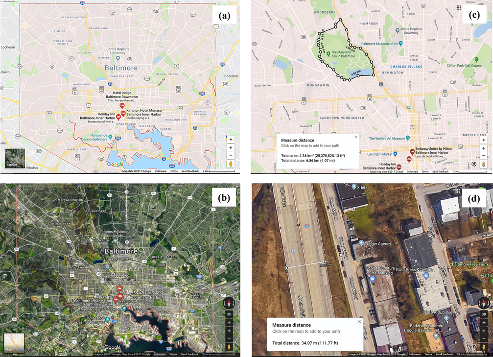

Close

Fig. 1

(a) Baltimore in Google Maps image, (b) Baltimore in Google Earth image, (c) area calculation by drawing polygons along the main road, and (d) measuring the width of a road (GoogleEarth, 2017).

Export to PPT

To calculate the width of the main street, we used the same procedures by selecting a starting point on one side of the street followed by “measure distance” instruction and then selecting the second point on the opposite side (Google Earth view). We also magnified the image so that 2 cm display represents 20 m actual distance. We used a very large number of residential areas for calculations to obtain much better confidence (mostly 100 residence areas).

4 Results and discussion

Table 1 shows the quantities belong to the examined cities. The last column shows the calculated critical fraction using Eq. (3). We were unable to obtain the TCL for Bandung, Nairobi, Kolkata, Mumbai, Limmasol, Timisoara, and Reykjavik and the NTI for Bandung, Tainan, Changsa, Buffalo, and Grand Rapids.

Based on congestion level (Tomtom, 2018), media and scientific reports (Batur et al., 2019; Çolak et al., 2016; Forbes, 2006; The Guardian, 2014, 2016; Times of India, 2018; Voanews, 2018), cities number 1–11 can be categorized as heavy traffic (congested) cities, while cities number 12–26 can be categorized as less congested cities. The Tomtom’s congestion level (TCL) of the congested city is likely above 35%, while the congestion level of the less congested city is below 35%. Further, the Numbeo traffic index (NTI) of the congested cities is likely above 160, while the traffic index of the less congested cities is below 160. If we look at the ${\rho }_{\text{c}}\text{/}{f}_{\text{c}}$ value (last column of Table 1), the congested cities have an ${\rho }_{\text{c}}\text{/}{f}_{\text{c}}$ value of below 0.1, while the less congested cities have an ${\rho }_{\text{c}}\text{/}{f}_{\text{c}}$ value of above 0.1. There seems to be a strong correlation between the Tomtom congestion level (2018) and the Numbeo traffic index (2018) on one hand and the fraction of a city’s critical areas on the other hand.

Variation of the ${\rho }_{\text{c}}\text{/}{f}_{\text{c}}$ on the $D_r\text{/}{D}_s$ ratio is shown in Fig. 2(a), where the ${\rho }_{\text{c}}\text{/}{f}_{\text{c}}$ decreases with increasing $D_r\text{/}{D}_s$ ratio. Lower ${\rho }_{\text{c}}\text{/}{f}_{\text{c}}$ represents easiness of congestion. Even with a small number of vehicles, the congested state still occurs. The lower ${\rho }_{\text{c}}\text{/}{f}_{\text{c}}$ is due to the less number of roads in a city, which means the city is dominated by residential regions. The average effective diameter of the residential areas is very large and when all vehicles originated from residential areas are using the roads, traffic stagnation occurs. In contrast, a large ${\rho }_{\text{c}}\text{/}{f}_{\text{c}}$ is obtained in cities with many roads. In these cities, the size of the residential areas is not large and the number of representative roads is very high. In Fig. 2(b), we also show the position of Mexico City, Moscow, Jakarta, Bandung, Kolkata, Bangkok, Baltimore, Vienna, Stuttgart, Berlin, Paris, and Indianapolis. It is clear from the figure that the ${\rho }_{\text{c}}\text{/}{f}_{\text{c}}$ of congested cities is smaller than 0.1, while the less congested cities have a ${\rho }_{\text{c}}\text{/}{f}_{\text{c}}$ of greater than 0.1. From the examined cities, Indianapolis has the highest ${\rho }_{\text{c}}\text{/}{f}_{\text{c}}$, which means that Indianapolis is the least congested city. This is consistent with its TCL (2018) of only 11%. In contrast, Bangkok has a very low ${\rho }_{\text{c}}\text{/}{f}_{\text{c}}$. This indicates that Bangkok is one of the most congested cities, which is consistent with its high TCL (2018) of 61%.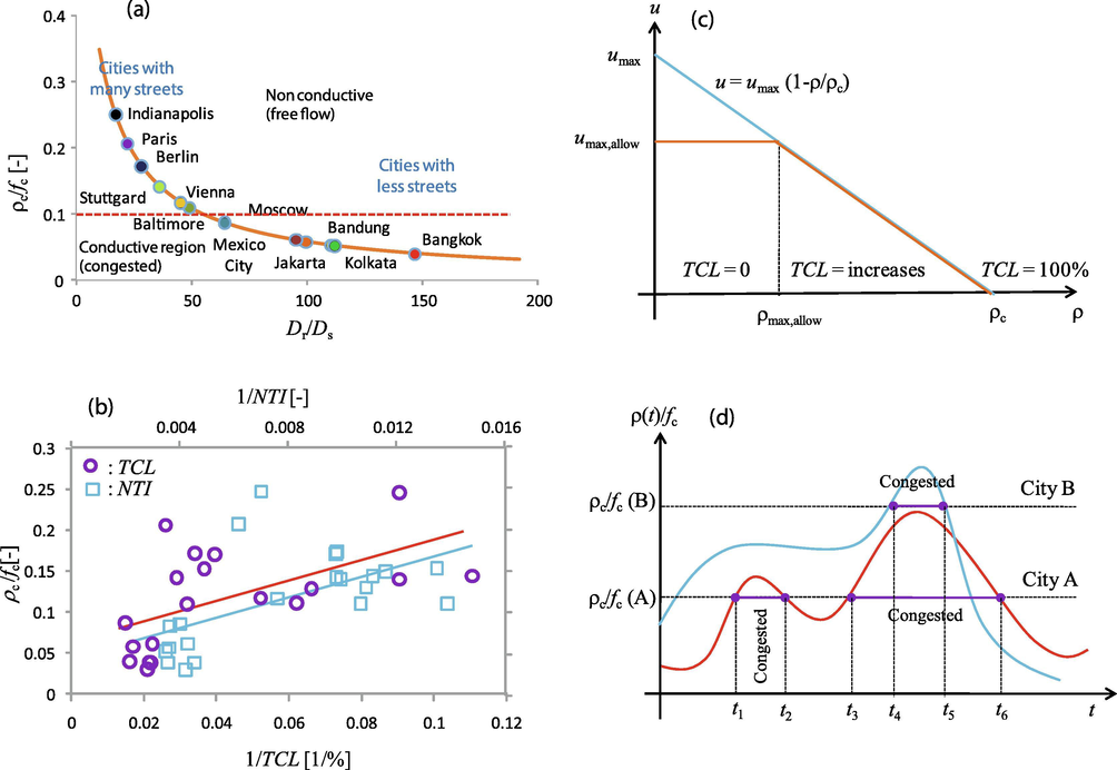

Close

Fig. 2

(a) Variation of the ${\rho }_{\text{c}}\text{/}{f}_{\text{c}}$ on the $D_r\text{/}{D}_s$ ratio and the corresponding figure for several cities. (b) The horizontal axis represents: (bottom) the inverse of Tomtom congestion level (2018), (top) the inverse of Numbeo traffic index (2018), and the vertical axis is the calculated ${\rho }_{\text{c}}\text{/}{f}_{\text{c}}$ (last column of Table 1). (c) Proposed dependence of vehicle speed on the density. The blue curve is based on Eq. (9) only. The brown curve is assumed speed based on Eqs. (9) and (10). (d) Cities having low ${\rho }_{\text{c}}\text{/}{f}_{\text{c}}$ are very easy to enter the percolation condition even at low vehicle densities while cities having high ${\rho }_{\text{c}}\text{/}{f}_{\text{c}}$ are rarely enter the percolation condition even at relatively high vehicle densities.

Export to PPT

The TCL (2018) measured the additional time required by the driver to pass the road compared to the time required in the uncongested condition. It depends on the vehicle velocity. The data were collected during one year and the index was obtained after averaging the annual data. Suppose the measurement was conducted during T (one year) or several months approaching one year. If we look at Eqs. (5) and (6), the uncongested condition does not mean that the vehicle density is zero (the velocity is maximum) since zero density means that the vehicle is absent on the road. Therefore, uncongested must mean that the vehicle can move up to permitted maximum velocity on the road (indicated by traffic sign).

For a simple model, we select the Greenshields function to represent the dependence of velocity on density as (Greenshields et al., 1935)

The modification of this model was proposed by Helbing and Tilch (1998) by introducing a more general relationship, $u=u_{max}{\left(1-{(\rho /{\rho }_c)}^{l-1}\right)}^{1/(1-m)}$ with a best fit was obtained using $l\approx 2.8$ and $m\approx 0.8$. Suppose the permitted maximum velocity at the $u_{max,allow}$, then the corresponding maximum density of vehicle so that the driver can drive up to this permitted velocity is ${\rho }_{max,allow}$ satisfies

This means that, even the vehicle density, $\rho$, is much lower than ${\rho }_{max,allow}$ or $0⩽\rho ⩽{\rho }_{max,allow}$, the speed must not exceed $u_{max,allow}$, or $0⩽u⩽u_{max,allow}$. Fig. 2(c) illustrates the speed of vehicle as a function of density based on Eq. (9) only (blue curve) and based on combined Eq. (9) and (10). This shape was also discussed by Jiang et al. (2001). The presence of flat section at low density was also discussed by Wang et al. (2011). If based on Eq. (9) only, we have one straight line that maximum at $\rho =0$ and zero at ${\rho }_c$. However, by using a combination of Eq. (9) and (10) we attain the speed is constant at $u_{max,allow}$ when $0⩽\rho ⩽{\rho }_{max,allow}$ and decreases according to Eq. (9) when $\rho >{\rho }_{max,allow}$.

The minimum time required by the driver to pass the road of length L in the uncongested condition becomes

However, in real situation, the velocity of the vehicle is approximated with Eq. (9) so that the time required by the vehicle to pass a road of length L in real situation is

Therefore, the additional time required by the driver becomes $\mathrm{\Delta }t=t_{\mathit{real}}-t_{\mathit{uncong}}$. We can show easily the following result$$\frac{\mathrm{\Delta }t}{T}=\frac{L/T}{u_{max}({\rho }_c-{\rho }_{max,allow})}〈\frac{(\rho -{\rho }_{max,allow})}{(1-\rho /{\rho }_c)}〉$$

But we must keep in mind that when the calculation results $\mathit{TCL}<0$ (caused by $\rho <{\rho }_{max,allow}$), the TCL must be adjusted to 0 since in that situation the density of the vehicle is less than the density for driving at the maximum allowed speed. Therefore, all vehicles are assumed to drive at that maximum allowed speed. The upper bound of the vehicle density so that the TCL is zero is when $〈\frac{(\rho -{\rho }_{max,allow})}{(1-\rho /{\rho }_c)}〉=0$. In the case of city having $\rho <<{\rho }_c$ we approximate

Therefore, the upper bound of the city to have zero TCL is $〈\rho 〉={\rho }_{max,allow}$. It is clear from Eq. (15) that the TCL increases with the average vehicle density $〈\rho 〉$, approximately linearly at low vehicle density. The TCL is also dependent on the traffic rule in the city since different city might have different $u_{max,allow}$ to mean different ${\rho }_{max,allow}$. If $u_{max,allow}$ in a city is low (${\rho }_{max,allow}$ is low), the TCL will be very high even the vehicle density is low but has surpassed ${\rho }_{max,allow}$.

Now, let us compare this prediction with data in Table 1. To investigate the relation of TCL with ${\rho }_c$. We can rewrite Eq. (15) as

We just need to inspect how TCL changes with ${\rho }_c$. For a rough investigation, let us assume other parameters are nearly constant so that the above equation can be approximated as $y=a+bx$ with $x=1/TCL$, $y={\rho }_c/f_c$, $a={\rho }_{max,allow}/f_c$, and $b=\kappa \left(〈\rho 〉-{\rho }_{max,allow}\right)/f_c$. We fit the data in Table 1 with Eq. (16). The result is shown in circle symbols in Fig. 3(b). The best fitting line (even if they seem scattered) resulting $y=0.065+1.171x$. Based on Table 1, the demarcation of the congested and less congested cities is at ${\rho }_{\text{c}}\text{/}{f}_{\text{c}}\approx 0.1$. Using this data, the demarcation of the TCL for congested and less congested cities is around $\mathit{TCL}\approx 33.5\%$, which is consistent with the TCL for Stuttgart of 34 (2018) which is located at the demarcation of the congested and less congested cities.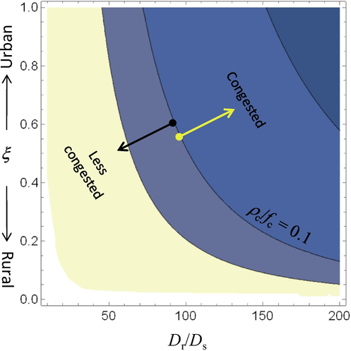

Close

Fig. 3

Contour plot of ${\rho }_{\text{c}}\text{/}{f}_{\text{c}}$ from Eq. (3) as function of $D_r\text{/}{D}_s$ and $\xi$. Curve with ${\rho }_{\text{c}}\text{/}{f}_{\text{c}}=0.1$ is a curve separating the congested (upper) and less congested (lower) cities.

Export to PPT

If we assume that the Numbeo traffic index (NTI) also satisfies the similar relation with $x=1/NTI$ and $y={\rho }_c/f_c$, we obtain the fitting equation, $y=0.044+9.142x$. Again, using the demarcation of the congested and less congested cities is at ${\rho }_c\approx 0.1$, we obtain the demarcation of the NTI (2018) is $\approx 163$. This is also consistent with data in Table 1 where the highest NTI for less congested city is Paris with NTI is 161. All congested cities have NTI of above 200. Surprisingly, the ${\rho }_{\text{c}}\text{/}{f}_{\text{c}}$, values in both fittings are nearly the same (0.065 and 0.044) although no adjustment was performed.

Mexico City, Moscow, Jakarta, Bandung, Kolkata, and Bangkok are the most congested cities, while Baltimore, Vienna, Stuttgart, Berlin, Paris, and Indianapolis are less congested cities. The first mentioned cities are very easy to enter the percolation condition (jamming) since the percolation thresholds are low while the later mentioned cities are rarely entering the percolation condition since the percolation thresholds are high. Even at low vehicle densities, the first-mentioned cities have entered the percolation condition while the later mentioned cities might stay at free flow condition at relatively high vehicle densities as illustrated in Fig. 2(d).

As shown in Eq. (8), a city is classified into congested or less congested depends also on the density of vehicles in the city. Rural city has very low vehicle density $\left(\xi <<1\right)$ so that even the ratio of residential area size to the road width is high, the congestion rarely occurs. To the contrary, the urban city having high vehicle density $\left(\xi \to 1\right)$ will easily enter the congestion condition. Fig. 3 shows the contour plot of ${\rho }_{\text{c}}\text{/}{f}_{\text{c}}$ from Eq. (3) as function of $D_r\text{/}{D}_s$ and $\xi$. The congested and less congested cities are separated by a curve with ${\rho }_{\text{c}}\text{/}{f}_{\text{c}}=0.1$. The region below this curve belongs to less congested cities, while that above this curve belongs to congested cities. The curve with ${\rho }_{\text{c}}\text{/}{f}_{\text{c}}=0.1$ satisfies the equation $\xi =5184/{\left(D_r/D_s\right)}^2$. In a very isolated region having a very low vehicle density $\left(\xi \to 0\right)$, the congestion never occurs. Theoretically, the congestion occurs when $D_r\text{/}{D}_s\to \infty$.

It seems that the proposed model is able to identify the congestion level of several cities around the world. The main parameter is the ratio between residential area and road width. Congested cities, such as populous cities in developing countries, have a large ratio of residential area to road width, while less congested cities have a small ratio of residential area to road width. Defining this parameter is very important to capture the strong relationship between landscape percolation and congestion. These findings may help in designing new cities or redesigning the infrastructure of congested cities, for example, for deciding what the maximum size of the residential area is and how width the roads are. This could be a good suggestion for the planners and policymakers to get an efficient and high accessibility city, a new mitigation analysis to reduce traffic congestion. Decisions on transport infrastructure have an impact that lasts for decades, even centuries, therefore they require analysis from various aspects. On the one hand, the planning and financing of transport infrastructure is a controversial political subject at the national and international levels (Short and Kopp, 2005). Indeed, the analysis of traffic jam mitigation is a complex system that must be understood in a broader element, from the traffic system, city dynamics, infrastructure management, land use, city geometry, economic growth, urban planning to the political context (Barthelemy, 2017; ECMT, 2007; Ramalho and Hobbs, 2012; Taylor, 2004; Turner et al., 2007).

5 Conclusion

The model of landscape percolation has been successfully applied to describe the traffic percolation in several populous cities around the world. We strongly identified that the congested condition of cities depends on the ratio of residential area to road width. After defining the area fraction of road, we obtained a criterion separating congested and less congested cities, i.e. the area fraction of about 0.1. Cities with an area fraction of less than 0.1 are classified as congested cities, while cities with area fraction of above 0.1 are classified as less congested cities. The conclusion is supported by several statistical data regarding the traffic conditions of cities around the world such as the Tomtom congestion level and the Numbeo traffic index.

References

- The effect of arbitrary stopping of public vehicles on flow of traffic in one-line streets. J. Teknol.. 2007;47(C):9-20.
- [Google Scholar]
- Ardekani, S.A., Williams, J.C., Bhat, S., 1992. Influence of urban network features on quality of traffic service. Transp. Res. Rec. 1358, 6–12.
- A global take on congestion in urban areas. Environ. Plann. B Plann. Des.. 2016;43(5):800-804.
- [CrossRef] [Google Scholar]
- Barthelemy, M., 2017. From paths to blocks: New measures for street patterns. Environ. Plan. B Urban. Anal. City Sci. 44(2), 256–271. https://doi.org/10.1177/0265813515599982.
- Self-organization versus top-down planning in the evolution of a city. Sci. Rep.. 2013;3:2153.
- Cities and Complexity. Cambridge, MA: MIT Press; 2005.
- Impact assessment of supply-side and demand-side policies on energy consumption and CO2 emissions from urban passenger transportation: the case of Istanbul. J. Clean. Prod.. 2019;219:391-410.
- Extent of capacity loss resulting from pavement distress. Proc. Inst. Civil Eng. Transp.. 2005;158(TR1):27-32.
- Mathematical Analysis of Urban Spatial Networks. Berlin and Heidelberg: Springer; 2009.
- Spatial information and the legibility of urban form: big data in urban morphology. Int. J. Inf. Manage.. 2019;102013
- Optimal reblocking as a practical tool for neighborhood development. Environ. Plan. B Urban Anal. City Sci.. 2019;46(2):303-321.
- Brelsford, C., Martin, T., Hand, J., Bettencourt, L.M.A., 2015. The topology of cities. Santa Fe Institute Working Papers (15-06-021), http://www.santafe.edu/media/workingpapers/15-06-021.pdf (Accessed 12 April 2020).
- Effect of road roughness on capacity of two-lane roads. J. Transp. Eng.. 2004;130(3):360-364.
- Effect of lane width on capacity under mixed traffic conditions in India. J. Transp. Eng.. 2003;129(2):155-160.
- Understanding congested travel in urban areas. Nat. Commun.. 2016;7(1):1-8.
- ECMT, 2007. Managing Urban Traffic Congestion. European Conference of Ministers of Transport (ECMT) Publishing, France
- An extended continuum traffic model with the consideration of the optimal velocity difference. Phys. A Stat. Mech. Appl.. 2018;508:402-413.
- Universal rules for fragmentation of land by humans. Landscape Ecol.. 2008;23:10131022.
- Forbes, 2006. India most congested cities. https://www.forbes.com/2006/12/19/india-most-congested-cities-biz-energy-cx_rm_1219congested.html#656ae09d678f (Accessed 8 January 2018)
- Impact of highway consistency on capacity utilization of two-lane rural highways. Can. J. Civil Eng.. 1999;26(6):789-798.
- GoogleEarth, 2017. https://www.google.com/earth (Accessed December 2017).
- The percolation phase transition in sea ice. Science. 1998;282:2238-2241.
- Governing. 2018. Governing, the states and legalities. governing.com (Accessed 25 February 2018)
- Gwyddion.net, 2018. After completely calculating and processing the data of 26 cities using the aforementioned method, we realized that there is a software to calculate area measurements faster, namely Gwyddion. However, in this work we just recalculated the residential area size using Gwyddion and showed the closeness of the results with data obtained by previous method. We did not further process the data obtained using Gwyddion because the final results will be the same, with only very slight deviations.
- Effect of highway geometric characteristics on capacity loss. J. Transp. Syst. Eng. IT. 2012;12(5):12-21.
- Generalized force model of traffic dynamics. Phys. Rev. E. 1998;58(1):133.
- Hume, C., 2017. Why traffic jams are a good thing. The Star, July 11, https://www.thestar.com/news/gta/2017/07/11/why-traffic-jams-are-a-good-thing.html (Accessed 12 April 2020).
- A new dynamics model for traffic flow. Chin. Sci. Bull.. 2001;46(4):345-348.
- Breakdown in Traffic Networks. Springer, Berlin: Fundamentals of Transportation Science; 2017.
- Estimation of capacity of two-lane two-way highways using simulation model. J. Transp. Eng. ASCE. 2010;136(1):61-66.
- The City Assembled: The Elements of Urban form through History. Boston: Little, Brown; 1999.
- Scaling laws in the spatial structure of urban road networks. Phys. A Stat. Mech. Appl.. 2006;363(1):89-95.
- Percolation transition in dynamical traffic network with evolving critical bottlenecks. Proc. Natl. Acad. Sci. USA. 2015;112(3):669-672.
- Urban freeway congestion: quantification of the problem and effectiveness of potential solutions. ITE J.. 1987;57(1):27-32.
- Lutenegger, B., 2018. Is traffic congestion a good thing? State Smart Transportation, June 18, https://www.ssti.us/2018/06/is-traffic-congestion-a-good-thing/ (Accessed on 12 April 2020).
- m.detik.com, 2017 (Accessed 25 February 2018).
- MA23. 2017. Vienna in Figures 2017 MA23, https://www.wien.gv.at/statistik/pdf/viennainfigures-2017.pdf (Accessed 25 February 2018)
- Influence of particle size on the electrical resistivity of compacted mixtures of polymeric and metallic powders. J. Appl. Phys.. 1971;42:614.
- Limited urban growth: London’s Street Network Dynamics since the 18th Century. Plos One. 2013;8(8):e69469
- Miller, B.G., 2011. The effect of coal usage on human health and the environment. In: Clean Coal Engineering Technology, Oxford, Butterworth-Heinemann
- Nakamura, M., 1994. Research and application of highway capacity in Japan. In: 2nd International Symposium on Highway Capacity, Sydney, Australia, 103–112
- Numbeo, 2018. Numbeo traffic index. https://www.numbeo.com/traffic/rankings.jsp (Accessed January 2019).
- Flow and capacity characteristics on two-lane rural highways. Transp. Res. Rec.. 1991;1320:128-134.
- Time for a change: dynamic urban ecology. Trends Ecol. Evol.. 2012;27:179-188.
- Empirical analysis of urban road traffic network: A case study in Hangzhou city, China. Phys. A Stat. Mech. Appl.. 2019;527:121287
- Transport infrastructure: investment and planning. Policy and research aspects. Transp. Policy. 2005;12(4):360-367.
- Price of anarchy is maximized at the percolation threshold. Phys. Rev. E. 2015;91(5):052126
- Elementary processes governing the evolution of road networks. Sci. Rep.. 2012;2:296.
- Stochastic cell transmission model (SCTM): a stochastic dynamic traffic model for traffic state surveillance and assignment. Transp. Res. Part B. 2011;45(3):507-533.
- The Guardian, 2014. Mumbai verge imploding polluted megacity. https://www.theguardian.com/cities/2014/nov/24/mumbai-verge-imploding-polluted-megacity (Accessed 8 January 2018)
- The Guardian, 2016. No escape – Nairobi air pollution. https://www.theguardian.com/cities/2016/jul/10/no-escape-nairobi-air-pollution-sparks-africa-health-warning (Accessed 8 January 2018)
- Times of India, 2018. Kolkata loses crores in traffic jam. https://timesofindia.indiatimes.com/city/kolkata/Kolkata-loses-crores-in-traffic-jams/articleshow/50816895.cms (Accessed 8 January 2018)
- Tomtom, 2018. Tomtom traffic index. https://www.tomtom.com/en_gb/trafficindex/list?citySize=LARGE&continent=ALL&country=ALL (Accessed January 2019)
- The politics of congestion mitigation. Transp. Policy. 2004;11(3):299-302.
- Reducing growth in vehicle miles traveled: Can we really pull it off? In: Sperling Daniel, Cannon James S., eds. Driving Climate Change Cutting Carbon from Transportation. Cambridge, MA: Academic Press; 2007. p. :129-142.
- City size, network structure and traffic congestion. J. Urban Econ.. 2013;76:1-14.
- The emergence of land change science for global environmental change and sustainability. Proc. Natl. Acad. Sci. USA. 2007;104:20666-20671.
- Navier-Stokes-like equations for traffic flow. Phys. Rev. E. 2005;72(4):046102
- Voanews, 2018. Nairobi traffic nightmare. https://learningenglish.voanews.com/a/nairobi-traffic-nightmare-sleepless-pupils/2866738.html (Accessed 8 January 2018).
- Percolation properties in a traffic model. Europhys. Lett.. 2015;112:38001.
- Logistic modeling of the equilibrium speed–density relationship. Transp. Res. Part A. 2011;45(6):554-566.
- Solving traffic congestion through street renaissance: a perspective from dense Asian cities. Urban Sci.. 2019;3(1):18.
- A dynamic and automatic traffic light control expert system for solving the road congestion problem. Expert Syst. Appl.. 2008;34(4):2370-2381.
- Estimation of origin–destination matrices for mass event: acase of Macau Grand Prix. J. King Saud Univ. Sci.. 2011;23(3):281-292.
- Modeling the growth of transportation networks: A comprehensive review. Netw. Spat. Econ.. 2009;9:291-307.
- Classification and unification of the microscopic deterministic traffic models. Phys. Rev. E. 2015;92(4):042802
- The marginal decrease of lane capacity with the number of lanes on highway. Proc. Eastern Asia Soc. Transp. Stud.. 2005;5:739-749.