

Translate this page into:
Investigation of soil moisture content over a cultivated farmland in Abeokuta Nigeria using electrical resistivity methods and soil analysis
⁎Corresponding author. ganiyusa@funaab.edu.ng (S.A. Ganiyu)
-
Received: ,
Accepted: ,
This article was originally published by Elsevier and was migrated to Scientific Scholar after the change of Publisher.
Peer review under responsibility of King Saud University.
Abstract
A combined 1D and 2D electrical resistivity surveys as well as laboratory determination of soil moisture contents of topsoil in a University cultivated farmland is presented. Apparent resistivity data were measured along six traverses using Schlumberger and Wenner arrays while soil samples were collected from all traverses at depths of 0.5, 1.0, 1.5 and 2.0 m respectively. The ranges of resistivity and thickness of the topsoil, clayey sand and weathered layers are 78.0–1094.0 Ωm, 0.5–1.9 m; 110.0–275.0 Ωm, 1.1–11.9 m; and 19.0–274.0 Ωm, 1.1–14.0 m respectively. 2D resistivity inverted sections revealed three zones of resistivity anomalies: topsoil with resistivity 78.0–600.0 Ωm for traverses within the farmland and that of two traverses along the entrances to the farm. The second resistivity zone represents a clay region of high moisture content with resistivity values less than 25.0 Ωm. The third layer represents weathered/fractured layer with relatively high resistivity values ranging from 116 to 600 Ωm. The 1D resistivity models showed effective depths of more than 30.0 cm while the 2D image lines revealed that active water uptake zone extends to about 3.0 m depth. All the collected soil samples belong to sandy loam while the soil moisture content values ranged from 45 to 74% at different soil depths of 0.5–2.0 m. The study has shown that the integrated methods provide important methods for better management of soil water reserves for improved agricultural production.
Keywords
2D resistivity imaging
Vertical electrical sounding
Farmland
Soil moisture content
Topsoil

1 Introduction
Good land management practices and environmental factors such as temperature, humidity, solar radiation and moisture content can influence crop growth (Jakalia et al., 2015). The information obtained from monitoring of soil water content in unsaturated zone is significant for planning irrigation schedule and minimizing lost yield due to soil salinity and water logging (Graham et al., 2013). Soil physical properties such as effective depth, texture and soil structure are important factors in determining suitability of soil for large scale production of cash crops such as oil palm (Mutert, 1999). The knowledge of variability of soil moisture content with depth and determination of rooting depth will provide a comprehensive understanding of the competition for soil water between annual and cash crops. Roots play a significant role in plant development and are responsible for various functions such as plant-soil water absorption, nutrient absorption, source of organic matter, storage, synthesis of growth substances among others (Basso et al., 2010). Thus, the availability of water at suitable effective depth for proper plant growth is of great importance to farming system. Therefore, in order to ensure an adequate water supply for growing crop on cultivated farmland, knowledge of soil moisture content as well as monitoring of its changes is of importance. Electrical resistivity method provides a non- destructive geophysical method for monitoring soil water dynamics from the surface to effective depth and beyond without soil disturbance (Mostafa et al., 2017). Electrical resistivity is strongly related to the amount of water content present in the soil. The resistivity of soil depends on saturation level, permeability, ionic concentration of the pore fluids and clay content (Abdel Aal et al., 2004). Thus, it is one of the most used geophysical methods for detecting changes in soil moisture content, groundwater flow pattern and an effective tool to determine depth to water saturated zone (Doser et al., 2004). Various geophysical methods have been employed to study soil water infiltration. Geo-electrical resistivity method is one of the geophysical methods that can be used to map and characterize spatial and temporal variations of soil physical properties (Sudha et al., 2009; Aizebeokhai, 2014). Electrical resistivity method is found to be cheap, quick and reliable for easy prediction of physical properties of soil (Dafalla and Al Fouzan, 2012) and for differentiating saline water zones (Majumdar and Pal, 2005; Narayanpethkar et al., 2006). Precipitation, seasonal variation in soil temperature, porosity, salinity, soil structure, air voids and changes in soil water content cause remarkable changes in the electrical conductivity of the soil (Benderitter and Schott,1999; Dafalla and Al Fouzan, 2012). Several researchers have employed the use of Electrical Resistivity survey especially 2D Electrical Resistivity Tomography (ERT) for agricultural purposes (Samouëlian et al., 2005; Amato et al., 2008; Srayeddin and Doussan, 2009; Basso et al., 2010; Nijland et al., 2010; Celano et al., 2011; Garré et al., 2013; Paglis, 2013). Soil analysis have been used to determine relationship between electrical resistivity of soil and moisture content (Abidin et al., 2014; Bhatt and Jain, 2014; Kowalczyk et al., 2014) while GPR and VES methods were used to identify boundaries of soil horizons and detect bedrocks at different degree of weathering process (Novàkovà et al., 2013). Vertical electrical sounding (VES) and 2D electrical resistivity tomography (ERT) are geo-electrical methods to understand subsurface lithology and delineate groundwater potential zones (Garcia-Montiel et al., 2008; Golekar et al., 2014). Scientists have also employed the use of either VES or 2D ERT in monitoring soil water content (Michot et al., 2003; Besson et al., 2004; Olayinka and Oladunjoye, 2005; Garcia-Montiel et al., 2008; Rings et al., 2008; Garre et al., 2012; Karim et al., 2013; Brilliante et al., 2015; Agunbiade and Ojoawo, 2014; Jakalia et al., 2015). The present study employed the integrated method of geophysical and soil analysis to investigate soil moisture distribution on a cultivated farmland. The study area is a farmland where several surface folder crops such as maize (Zea mays), cassava (Manihot esculenta) and yam (Dioscorea Alata) have been planted successfully with good quality harvests over the past few years. These annual crops can thrive well within the topsoil effective depth of 0–30.0 cm. The soil texture of the study area is suitable and support cultivation of these arable crops. Intercropping system is a form of agricultural cultivation system that can serves as possible risk reduction strategy for farmers as it allows for crop diversification, less chance of crop yield loss by various disease causing organisms and the potential complementary attitudes of the root systems of different crops in an effective soil water and nutrient use (Garré et al., 2013; Hairiah et al., 2000). There is no record of geophysical investigation work which aimed to provide information about variation of soil electrical conductivity with effective soil depth for cultivation of either cash or arable crops on the farmland. The objectives of the present study is to explore the integrated use of VES and 2D ERT to monitor the variation of soil water content with depth on the farmland, detect the effective depth that can support the growth of cash crops especially during dry season and evaluate the suitability of the farmland for intercropping system.
1.1 Description of the study area
The study area is an agricultural farm managed by Directorate of University Farms (DUFARMS), Federal University of Agriculture, Abeokuta (FUNAAB). The study area is located at Latitudes 7°14′4″N − 7°14′7″N with Longitudes 3°26′7″E − 3°26′10″E and lies within a forest-savanna transition zone in southwestern part of Nigeria (Fig. 1). Abeokuta experiences two local climates (rainy and dry seasons). The wet season starts from March-October while the dry season occurs from November-March when the area is under the influence of North-easternly winds (Badmus and Olatinsu, 2010). The amount of rainfall varies between 750 and 1000 mm in the rainy season and 250–500 mm during the dry season (Akanni, 1992). Abeokuta is characterized by an undulating topography with elevation value ranging from 100 to 400 m above sea level (Akanni, 1992; Oloruntola and Adeyemi, 2014). The mean monthly temperature ranges between 25.7 °C in July to 30.2 °C in February with the mean annual temperature of 26.6 °C.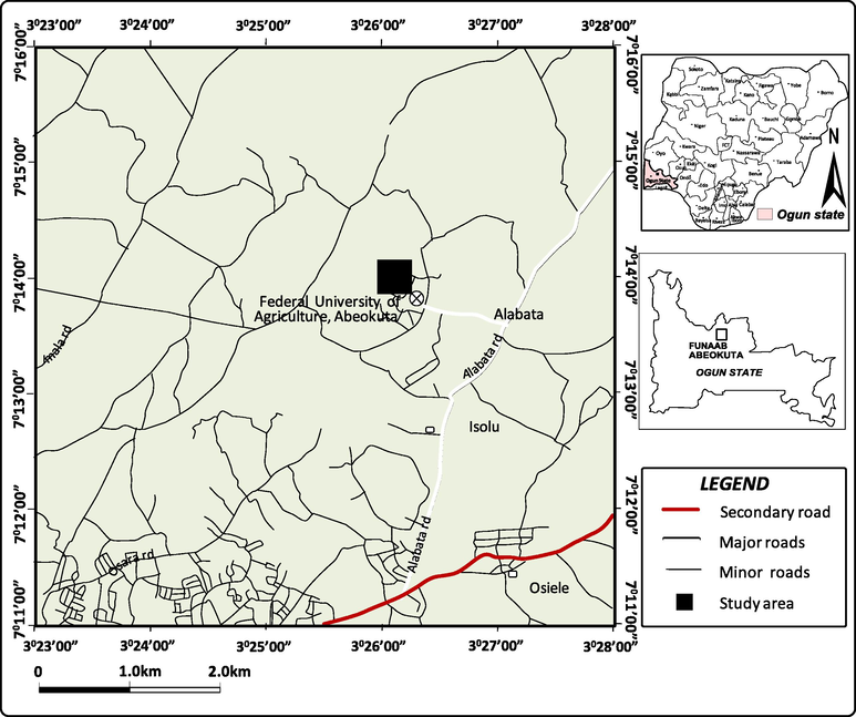
Map showing location of the study area.
1.1.1 Geology of the study area
The study area falls within the Basement Complex formation of southwestern Nigeria. Abeokuta is located on crystalline basement complex of igneous and metamorphic origin (Gbadebo et al., 2010). The basement rocks are of Precambrian age to early Paleozoic age and extend from the north-eastern part of Ogun state, of which Abeokuta belongs and dipping towards the coast (Ako, 1979). The basement complex rock comprises of coarse-porphyritic hornblende-biotite-granodiorite, biotite granite gneiss, pegmatite, porphyoblastic granite gneiss, quartz-schist and amphibolite/mica-schist (Jones and Hockey, 1964; Kehinde-Phillips, 1992). The foliation and joints on these rocks control the course of the two major rivers of Ogun and Oyan causing them to form trellis pattern. The prolonged weathering of the crystalline rock has led to the development of regoliths of varying thicknesses which ultimately reduced the conductivity of the parent rocks (Badmus and Olatinsu, 2012). The degree of weathering also depends on the depth of the rock beneath the earth surface. Abeokuta belongs to the stable plate which was not subjected to intense tectonics in the past, thus the underground faulting system is minimal (Ufoegbune et al., 2009). Abeokuta is also said to be part of the transition zones of the southwestern Nigeria. The northern side of Abeokuta is characterized by pegmatitic veins underlain by granite while the southern part enters the transition zone with the sedimentary formation of the eastern Dahomey Basin. The western part of Abeokuta is characterized by granitic gneiss of less porous nature together with various quartzite intrusions (Key, 1992). At the southeastern and southwestern parts of the area is the outlier of the ISE formation of Abeokuta group which consist of conglomerates and grits at base and in turn overlain by a coarse medium grained loosed sand (Aladejana and Talabi, 2013). Outcrops of cross-bedded, ferruginous sandstones and pebbly sandstones have been noted near the base of the succession among the outliers south-east of Abeokuta (Jones and Hockey, 1964). The terrain of Abeokuta is characterized by two types of landforms, these are sparsely distributed low hills and knolls of granite, other rocks of basement complex and nearly flat topography (Adekunle et al., 2013). The soil of the study area is gravelly loamy sand underlain by undifferentiated basement complex of an alluvio-colluvial parent material (Busari and Salako, 2015). Taxonomically, the soil was classified as Arenic Plinthic Kandiudalf and Arenic Lixisol based on United State Department of Agriculture (USDA) and Food and Agricultural Organization (FAO)/United Nations Educational, Scientific and Cultural Organization (UNESCO) classification system respectively (Soil Survey Staff, 2006; FAO, 2015). The dominant rock type in the study area is migmatite gneiss. The geological map of the study area is shown in Fig. 2.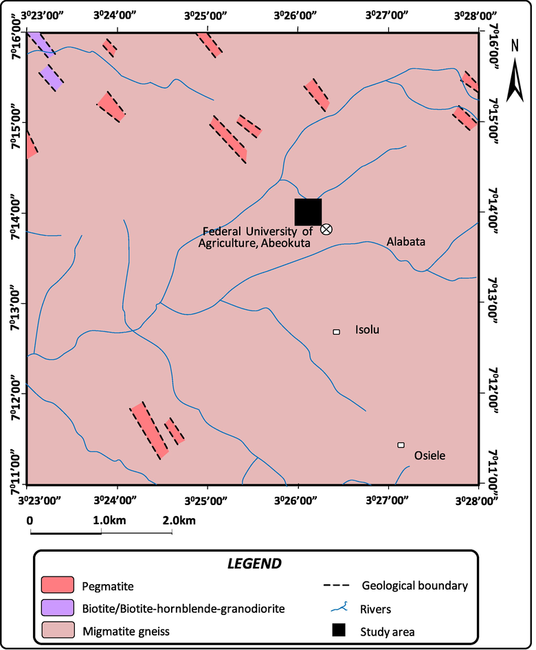
Geological map showing the rock type that underlies the study area (adapted from Jones and Hockey, 1964).
2 Methodology
2.1 Vertical electrical sounding (VES) survey
A total of six VES were carried out along the 2D profile lines laid within and outside the farmland using Campus Tigre Resistivity Meter in March 2016. Four lines were laid within the farmland in the E -W direction with a separation of 7 m between the image lines while the remaining two (2) profile lines with a separation distance of 48 m were measured along the entrances to the farm as shown in Fig. 3. The electrode arrangement employed for VES was Schlumberger with a maximum current electrode separation of 110 m. Each VES location was chosen at the middle of 2D profile line with a current electrode spread (AB/2) of 55 m. The VES resistivity data obtained on the field were partially curve matched before being computer iterated with WINRESIST software with a R.M.S error of less than 5.0 so as to obtain the true resistivity and layer parameters. The iterated geoelectric parameters obtained were used to generate geo-electric sections.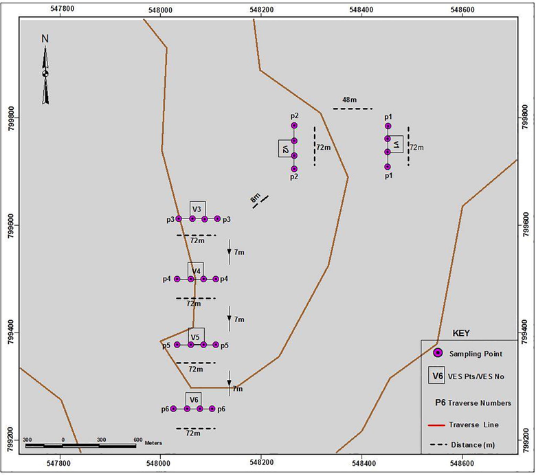
Field layout for the 2D Traverse Lines and VES Points.
2.2 2D electrical resistivity survey
2D Electrical Resistivity survey was also carried out within the seasonally cultivated farmland. The profiles layouts were as described for VES survey. Each 2D profile line was 72 m in length. The electrode arrangement employed for 2D ERT was Wenner array configuration. Fig. 3 shows the data acquisition map for resistivity survey. The electrode separation distance for each traverse ranged from a = 3 to 18 m with a station interval of 3 m. The 2D ERT raw data obtained on the field were inverted through the use of RES2DINV software (Loke and Barker, 1996). RES2DINV program automatically determines the 2D resistivity model of the subsurface from the input 2D resistivity data using the smoothness constrained least square method (Sasaki, 1992). The iterative optimization method attempted to reduce the differences existed between the measured resistivity values and calculated resistivity values with the inversion model. The accuracy of fit is expressed in terms of RMS error (Loke and Barker, 1996).
2.3 Soil samples Collection
Twenty four (24) soil samples were collected along the profiles at depths of 0.5, 1.0, 1.5 and 2.0 m respectively on each profile for laboratory analysis of particle size distribution and soil moisture content. Collection of soil samples at these depths should offer information on the estimated depth to the shallow water table within the farmland (Olayinka and Oladunjoye, 2005) and also assist in evaluating the suitability of the soil for cultivation of tree crops with effective depths greater than 30 cm of most arable crops. Soil samples were collected with the aid of soil auger and core samplers. The collected soil samples were analyzed in soil laboratory of the Department of Soil Science and Land Management of FUNAAB, Nigeria. The particle size analysis of the collected air dried soil samples was done according to the procedures outlined by Gee and Bauder (1986) with the help of hydrometer method while the textural classification was done using the USDA textural soil classification system. Soil moisture content was determined using the weight loss method based on ASTM D4959-07 standard.
3 Results and discussion
3.1 VES result
The results obtained from the VES are shown in Fig. 4. The study area is underlain by three or four layers of varying lithologies. Two resistivity sounding curve types were obtained and are mostly H-types
except at VES 1 which have KH type
. The range of the values of thicknesses of each layer for all the six VES points are given as: Topsoil ranges between 0.5 and 1.3 m, clayey sand layer between 1.1 and 11.9 m and weathered basement between 1.1 and 14.0 m. This is shown in Table 1.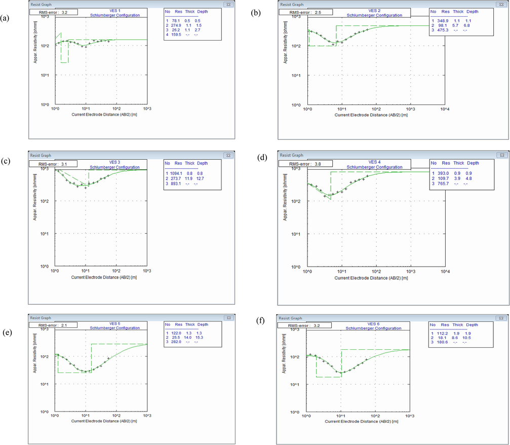
Layer model interpretations for VES 4, VES 5 and VES 6.
Station
Layer no
Resistivity value (Ωm)
Thickness (m)
Depth (m)
Curve type
Reflection coefficient
Probable lithology
VES 1
1
78
0.5
0.5
Topsoil
2
275
1.1
1.6
KH
0.72
Clayey sand
3
26
1.1
2.7
clay
4
160
–
–
Fractured basement
VES 2
1
349
1.1
1.1
Topsoil
2
98
5.7
6.8
H
0.65
clay
3
475
–
–
Fractured basement
VES 3
1
1094
0.8
0.8
Topsoil
2
274
11.9
12.7
H
0.53
Clayey sand
3
893
–
–
Fractured basement
VES 4
1
393
0.9
0.9
Topsoil
2
110
3.9
4.8
H
0.75
Clayey sand
3
766
–
–
Fractured basement
VES 5
1
122
1.3
1.3
Topsoil
2
26
14.0
15.3
H
0.83
clay
3
282
–
–
Partially fractured basement
VES 6
1
112
1.9
1.9
Topsoil
2
18
8.6
10.5
H
0.82
Clay
3
181
–
–
Partially fractured basement
The topsoil resistivity values ranged from 78.0 to 1094.0 Ωm while the layer thickness ranged from 0.5 to 1.9 m. The range of resistivity values obtained for the topsoil for VES 1, 2, 5 and 6 were between 78.0 and 349.0 Ωm which is within that of sandy-loam soil class (Loke et al., 2004) while VES 3 has topsoil resistivity values of 1094.0 Ωm. The variations in topsoil resistivity could be as a result of different degree of compaction due to reworking activities at the farmland. The clayey sand layer resistivity values range from 110.0 to 275.0 Ωm with thickness values from 1.1 to 11.9 m. The weathered basement resistivity values lie between 19.0 and 274.0 Ωm while the layer thickness varies between 1.1 and 14.0 m. The fractured basement has resistivity values ranging between 160.0 and 893.0 Ωm. fractured basement columns were delineated beneath VES 1, 2, 3 and 4 while partially fractured basement were delineated beneath VES 5 and 6.
From the VES results, relatively thin sandy loam/sandy clay loam constitutes the topsoil of the study area.
3.2 Geo-electric section
The lateral and vertical variation in depth and thickness of the subsurface layers was revealed with the aid of geo-electric sections. The sections showed that the study area is underlain by geologic sequence consisting of the topsoil, thin clayey sand, sandy clay and fractured basement.
3.2.1 Cross section between VES 1 and 2
The cross section between VES 1 and 2 that serves as entrances to the farm is presented in Fig. 5a. It showed that the study area is underlain by four layers representing the topsoil, clayey sand, sandy clay and fractured basement. The first two units in the section is the overburden with resistivity and thickness values ranging from 78.0 to 349.0 Ωm/0.5 to 1.1 m and 26.0 to 98.0 Ωm/1.1 to 5.7 m respectively. The lowermost fractured basement resistivity values ranged from 160.0 to 475.0 Ωm.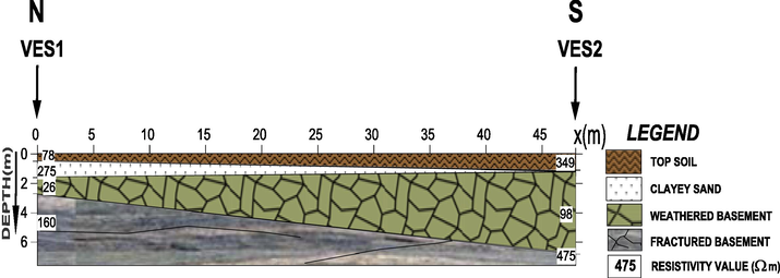
Cross section between VES 1 and 2.
The topsoil layer has a near surface horizontal geometry while the weathered layer (predominantly clayey) has its thickness increasing towards the southern end of the profile.
3.2.2 Geo-electric section across VES 3, 4, 5 and 6
Fig. 5b represents the geoelectric section across the profiles within the farmland. The resistivity of the topsoil ranges from 112.0 to 1094.0 Ωm while that of the weathered basement ranges from 18.0 to 274.0 Ωm. The weathered layer (clay) with resistivity value less than 30.0 Ωm in both VES 5 and 6 are similar while that of VES 3 and 4 (clayey sand) are also identical in nature. The fractured basement resistivity value varies from 181.0 to 893.0 Ωm. The topography of this section is uneven with thickness range of 3.9–14.0 m and depth range of 4.8–15.3 m. The basement is much closer to the surface with a depth of 4.8 m occurring at offset 7.0 m towards the east axis. The fractured basement model resistivity is less than 500 Ωm in VES 5 and 6 justifying the incompetent and fractured nature (Aina et al., 1996). The resistivity values of fractured layer beneath VES 3 and 4 is >500 Ωm. The highest resistivity value of fractured layer with 893.0 Ωm occurs at VES 3.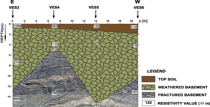
Geo-electric section across VES 3, 4, 5 and 6.
3.3 Interpretation of 2D resistivity models
Fig. 6a−f show the inverse model sections of the subsurface and resistivity distribution derived from the 2D inversion of resistivity data. As shown in Fig. 6a, the resistivity-depth model shows relatively high resistivity variation on the near surface almost along the entire traverse. This may be due to high evaporation rate, high stiffness value and untilled state of the farm during the time of surveying. The resistivity of the top soil layer from the 2D resistivity model ranged from 176.0 to 600.0 Ωm up to a depth of about 3 m. This is an indication of unsaturated topsoil (loamy sand) with low soil moisture content. The first layer, which was 0.5 m thick with resistivity of 78.1 Ωm was the topsoil from 1D model obtained from VES 1 (Fig. 4a). An isolated conductive zone of resistivity values less than 20.0 Ωm (clay rich layer/loam) was noticed at lateral distance of 12.0–21.0 m while another relatively low resistive region within the bedrock were noticed at lateral distance of 38.0–62.0 m along the profile. This corresponds with a layer below the topsoil of VES1 with a resistivity of 26.2 Ωm of clay (moist soil) nature. A relatively high resistivity value (174.0–516.0 Ωm) appears as a transition interval between two conducting zones at lateral distance of 19.0–38.0 m along the traverse. Fig. 6b shows model section for traverse 2 with the topsoil (loamy sand) characterized by resistivity values of 176.0–561.0 Ωm with thickness ranging from 0 to 2.0 m. The 1D model for VES 2 indicates topsoil (loamy sand) layer with a resistivity of 349.0 Ωm at a depth of 1.1 m. The second layer with resistivity values of 56.0–99.0 Ωm and thickness 2.2–3.6 m represent highly weathered layer. The third resistivity anomaly zone represent a continuous spread of conductive region with low resistivity values <25.0 Ωm almost along the entire traverse from about 4.0–8.0 m depth. This region serves as the clay rich zone. This corresponds to the clay layer below the topsoil of VES 2 with resistivity of 98.0 Ωm at a depth of 6.0 m. Fig. 6c shows the inverted section of traverse 3, at horizontal distance of 5.0–68.0 m, the near surface has resistivity values of 98.0–561.0 Ωm suggestive of sandy loam topsoil. This is an indication of unsaturated top soil and localized lateral resistivity inhomogeneities. At a depth of about 3.8–7.5 m, there is a continuous low resistive region along the entire length of the traverse. This represents the presence of clay rich region in saturated condition up to a depth of about 8.0 m. Below 8 m depth is the presence of a weathered/fractured layer with resistivity values 31.0–99.0 Ωm at a lateral distance 20.0–52.0 m.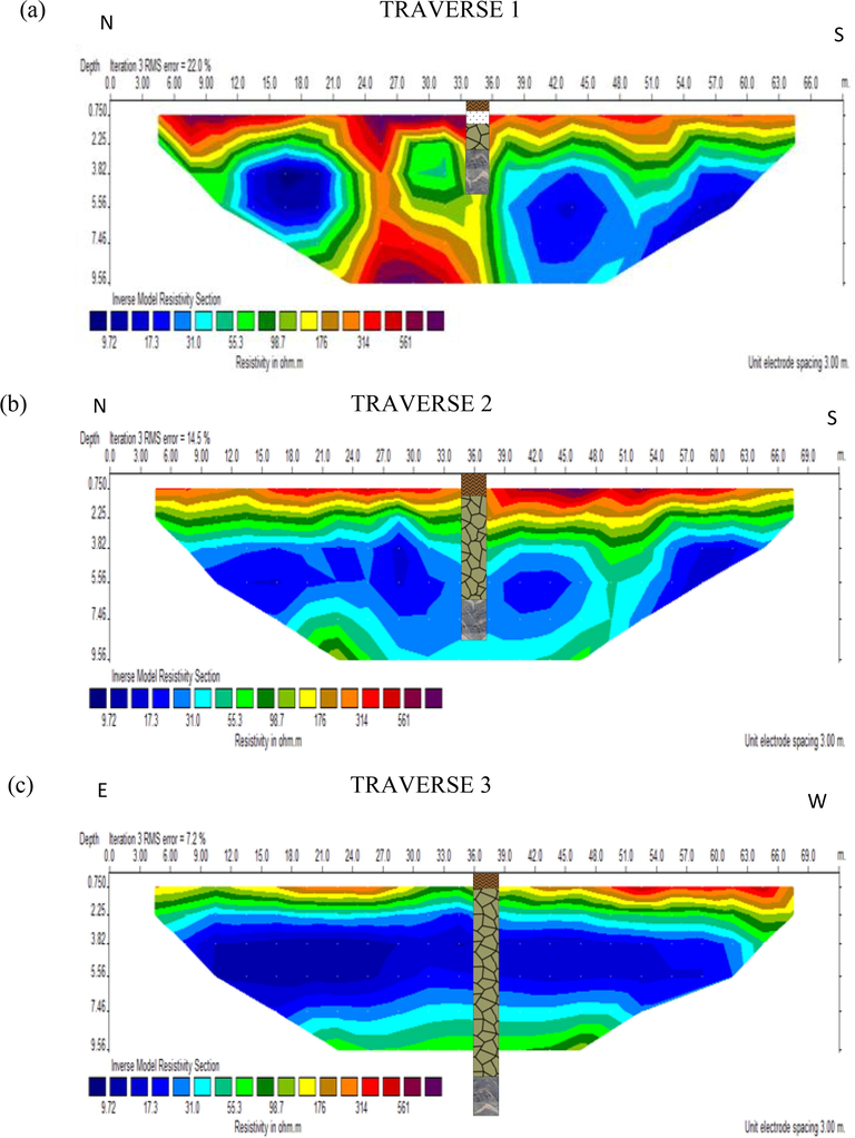
2D inverse resistivity model for traverses 1, 2 and 3.
2D inverse resistivity model for traverses 1, 2 and 3.
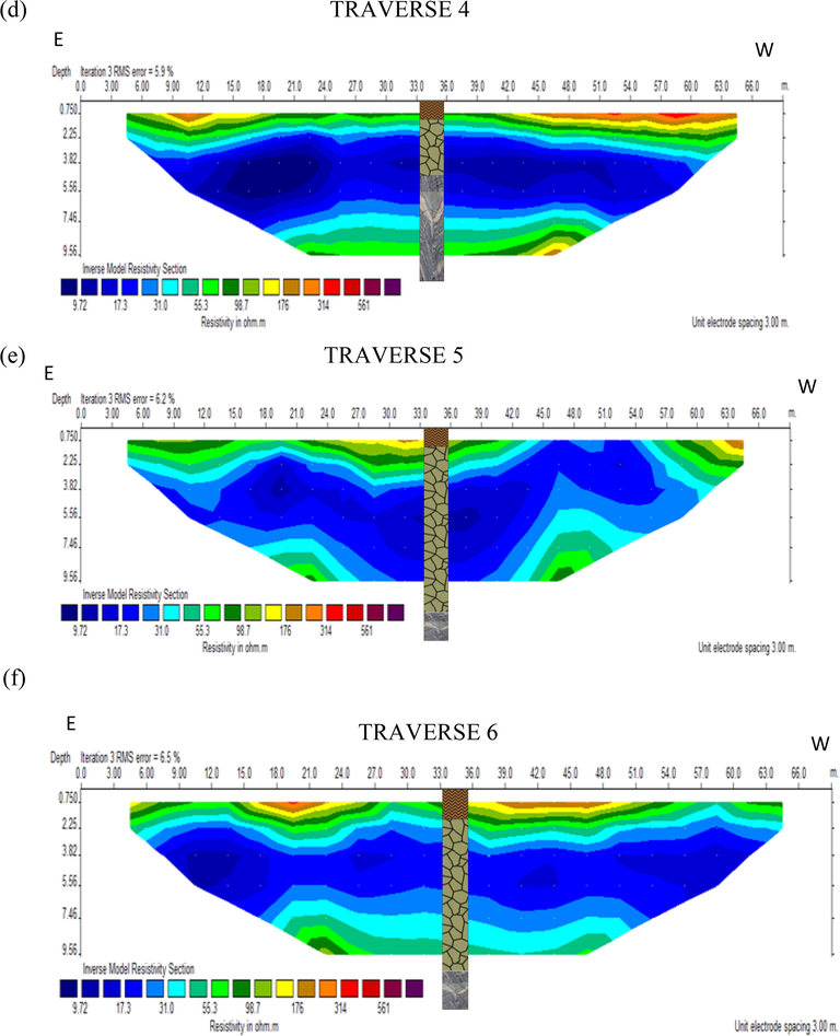
The inversion model of traverse 4 (Fig. 6d) depicts near surface resistivity anomaly (176.0–314.0 Ωm) suggestive of sandy loam/loamy sand topsoil at lateral distances 7.0–15.0 m and 42.0–65.0 m along the traverse at a depth of about 1.5 m. The 1D model of VES 4 showed topsoil with resistivity value of 393.0 Ωm at a depth of 0.9 m (Fig. 4d). This may be due to high evaporation rate and unsaturated near surface soil or untilled status of the soil during survey time. This was followed by clay/humid soil at a depth of about 3.8 m up to a depth of 8.0 m. The weathered/fractured layers have resistivity values ranging between 31.0 and 176.0 Ωm at lateral distance 20.0–54.0 m below a depth of 8.0 m. The maximum depth of investigation for the profile model was about 10 m. Fig. 6e shows inverse model section of traverse 5 in which resistivity values of 176.0–314.0 Ωm was noticed at lateral distance 25.0–36.0 m and 62.0–65.0 m towards the end of the traverse up to a depth of about 1.5 m. This is suggestive of topsoil/sandy clay/sandy loam nature. The 1D model for VES 5 indicates that the resistivity of topsoil is 122.0 Ωm at a depth of 1.3 m followed by a sandy clay zone with a resistivity of 26.0 Ωm at a depth of 15.0 m. Weathered layer was noticed in the 2D model at lateral distances 5.0–24.0 m and 37.0–44.0 m with resistivity values 56.0–99.0 Ωm. Low resistive region with resistivity value <20.0 Ωm protruded to the surface at position 45.0–55.0 m along the traverse. This was followed by clay/sandy clay material with resistivity values ranging between 56.0 and 99.0 Ωm. In Fig. 6f, the 2D resistivity model showed relatively high resistivity anomaly close to the surface with values of 176.0–314.0 Ωm, indicating sandy loam/loamy sand topsoil at lateral distances of 15.0–25.0 m and 34.0–52.0 m along the traverse. The 1D model of VES 6 (Fig. 4f) indicates that the resistivity of the topsoil layer is 112.0 Ωm followed by clay (18.0 Ωm) and fractured basement zones respectively. The 2D resistivity model showed clay/moist soil region of low resistivity anomaly values <20.0 Ωm which occurs throughout the entire traverse. This was noticed from a depth of about 3.8–7.5 m. Below the clay rich zone is the presence of fractured/weathered bedrock layer with resistivity values ranging between 56.0 and 99.0 Ωm at a depth of about 9 m.
It should be noted that the 2D resistivity models of traverses 1 and 2 showed continuous occurrence of high resistivity anomaly on topsoil. This may be due to the fact that the two profiles serve as entrances to the farm. The VES and 2D imaging revealed soil type and topsoil effective depths suitable for a well developed root systems of cash crops such as Oil palm (Elaeis guineensis) and Cocoa (Theobroma cacao) cultivation (Goh and Chew, 1994; Mutert, 1999; Ibiremo et al., 2011; Agunbiade and Ojoawo, 2014). The 2D models also show that the clay rich/moist soil zones were noticed at approximate depth of about 3.8–7.5 m for traverses 2, 3 and 4 while it extends from the near surface up to 10 m depth for traverse 5 at lateral distance 45.0–55.0 m along the traverse. Comparison between results of VES and 2D imaging showed that there is similarity in thickness and resistivity values for some electrical layers/horizons.
3.4 Soil samples analysis
Soil classification test using particle size distribution result showed that soils at cultivated farmland belong to Sandy loam (Table 2). This result agrees with earlier work by Elias and Gbadegesin (2012) who reported that dominant soil type of the basement complex rocks are loamy sand or sandy loam underlain by a variety of alluvial or colluvial materials over coarse-grained granitic gneiss and pegmatite.
S/N
Ves sample
Percentage of sand
Percentage of clay
Percentage of silt
Soil type
Average soil type
1
VES 01 SAMPLE 01
78.6
18.6
2.8
Sandy loam
Sandy loam
2
VES 01 SAMPLE 02
80.6
18.6
0.8
Sandy loam
3
VES 01 SAMPLE 03
80.6
16.6
28
Sandy loam
4
VES 01 SAMPLE 04
80.6
18.6
0.8
Sandy loam
5
VES 02 SAMPLE 01
80.6
18.6
0.8
Sandy loam
Sandy loam
6
VES 02 SAMPLE 02
78.6
16.6
4.8
Sandy loam
7
VES 02 SAMPLE 03
80.6
18.6
0.8
Sandy loam
8
VES 02 SAMPLE 04
80.6
18.6
0.8
Sandy loam
9
VES 03 SAMPLE 01
77.6
19.6
2.8
Sandy loam
Sandy loam
10
VES 03 SAMPLE 02
79.6
19.6
0.8
Sandy loam
11
VES 03 SAMPLE 03
76.6
19.6
3.8
Sandy loam
12
VES 03 SAMPLE 04
79.6
16.6
3.8
Sandy loam
13
VES 04 SAMPLE 01
80.6
18.6
0.8
Sandy loam
Sandy loam
14
VES 04 SAMPLE 02
78.6
18.6
2.8
Sandy loam
15
VES 04 SAMPLE 03
79.6
17.6
2.8
Sandy loam
16
VES 04 SAMPLE 04
77.6
18.6
3.8
Sandy loam
17
VES 05 SAMPLE 01
78.6
18.6
2.8
Sandy loam
Sandy loam
18
VES 05 SAMPLE 02
78.6
19.6
1.8
Sandy loam
19
VES 05 SAMPLE 03
77.6
19.6
2.8
Sandy loam
20
VES 05 SAMPLE 04
78.6
19.6
1.8
Sandy loam
21
VES 06 SAMPLE 01
75.6
19.6
4.8
Sandy loam
Sandy loam
22
VES 06 SAMPLE 02
74.6
18.6
6.8
Sandy loam
23
VES 06 SAMPLE 03
74.6
20.6
4.8
Sandy clay loam
24
VES 06 SAMPLE 04
72.6
20.6
6.8
Sandy clay loam
The values of soil moisture content at different soil depths of 0.5–2.0 m ranged from 45 to 74% (see Table 3). It was observed that the soil moisture content increases with depths for most of the traverses. This is in agreement with work of Halfmann (2005) and Olorunfemi and Fasinminri (2011). It was further observed that there is significant increase in soil moisture at 1.5–2.0 m depth. This corresponds with the transition from high resistivity near surface layer to relatively low resistivity weathered layer.
Depth (m)
Soil moisture content in % (Traverse 1)
Soil moisture content in % (Traverse 2)
Soil moisture content in % (Traverse 3)
Soil moisture content in% (Traverse 4)
Soil moisture content in% (Traverse 5)
Soil moisture content in % (Traverse 6)
0.5
45
49
51.5
50.2
51
51
1.0
48
52
52.2
50.5
54
54
1.5
50
66
52
71.5
55
55
2.0
59
72
61
74.0
70
68
4 Conclusions
The study has demonstrated the ability of the combined method of electrical resistivity surveys involving VES and 2D ERT with laboratory analysis of soil moisture content to effectively characterize soil and variations of soil moisture content with varying depths. Geoelectrical method of VES and 2D ERT allowed vertical and lateral delineation of soil horizons and serves as effective monitoring of soil structural heterogeneity. The maximum depth of investigation as observed from VES results is more than 14.0 m while that of the 2D model was about 10.0 m. The 2D ERT imaging revealed that clay rich zone (deep saturated soil layer) occurs at approximate depth of about 3.8–7.5 m for most of the traverses, thus defining a zone of relatively permanent water saturated condition. The deep saturated soil layer may provide moderate but vital water for evapotranspiration process when upper layer soil moisture stress reaches a maximum in the late dry/early wet season. The soil type and the estimated effective depths in the study area support cash crops cultivation which is more economical than most arable crops. However, further research work on analysis of physio-chemical properties of collected soil samples will assist to check if special land management techniques are required for optimal production of intending cash crops. The extent of reliability of the obtained effective depths as shown by resistivity models can be enhanced through the use of other geophysical methods such as Electromagnetic Induction and Induced Polarization which are also sensitive to moisture content.
References
- Effects of microbial processes on electrolytic and interfacial electrical properties of unconsolidated sediments. Geophys. Res. Lett.. 2004;31
- [CrossRef] [Google Scholar]
- Correlation analysis between field electrical resistivity value (ERV) and basic geotechnical properties (BGP) Soil Mech. Found. Eng.. 2014;51(3):117-125.
- [Google Scholar]
- Pollution studies on groundwater contamination: water quality of abeokuta, Ogun State, South-West Nigeria. J. Environ. Earth Sci.. 2013;3(5):161-166.
- [Google Scholar]
- Evaluation of effective soil depth and heterogeneous subsurface mapping using electrical resistivity geophysical method to aid oil palm plantation planning at Ile-Oluji, Ondo State, Nigeria. Am. J. Sci. Ind. Res.. 2014;6(3):58-68.
- [Google Scholar]
- An integration of aeromagnetic and electrical resistivty methods in dam site investigation. Geophysics. 1996;61(2):349-356.
- [Google Scholar]
- In situ detection of tree root distribution and biomass by multielectrode resistivty imaging. Tree Physiol.. 2008;28(10):1441-1448.
- [Google Scholar]
- Assessment of soil salinity using electrical resistivity imaging and induced polarization methods. Afr. J. Agric. Res.. 2014;9(45):3369-3378.
- [Google Scholar]
- C.O. Akanni, S.O. Oyesiku, and O.O Jegede, F.J (Eds.) published by Rex, Relief, drainage, soil and climate of Ogun state in maps(pp 6–20).In Onakomaiya 1992 Charles publication
- Geophysical Prospecting for Groundwater in Parts of South-Western Nigeria. Nigeria: Department of Geology, University of Ife, Ile-Ife; 1979. p. :p371. Unpublished PhD Thesis.
- Assessment of groundwater quality in Abeokuta, Southwestern Nigeria. Research inventory. Int. J. Eng. Sci.. 2013;2(6):21-31.
- [Google Scholar]
- ASTM D4959-07, Standard test method for determination of water (moisture) content soil by direct heating 2007 American society for testing materials, New York Annual book of ASTM standards
- Aquifer characteristics and groundwater recharge pattern in a typical basement complex, southwestern, nigeria. Afr. J. Environ. Sci. Technol.. 2010;4(6):328-342.
- [Google Scholar]
- Geophysical characterization of basement rocks and groundwater potentials using electrical sounding data from odeda quarry site, Southwestern. Asian J. Earth Sci.. 2012;5:79-87.
- [Google Scholar]
- Two dimensional spatial and temporal variations of soil physical properties in tillage systems using electrical resistivity tomography. Agronomy J.. 2010;102:440.
- [CrossRef] [Google Scholar]
- Short-time variation of the resistivity in an unsaturated soil: the relationship with rainfall. Eur. J. Environ. Eng. Geophys.. 1999;4:37-49.
- [Google Scholar]
- Structural heterogeneity of the soil tilled layers as characterized by 2D electrical resistivity surveying. Soil Tillage Res.. 2004;79:239-249.
- [Google Scholar]
- Correlation between electrical resistivity and water content of sand- a statistical approach. Am. Int. J. Res. Sci. Technol. Eng. Math.. 2014;6(2):115-121.
- [Google Scholar]
- The use of soil electrical resistivity to monitor plant and soil water relationship in Vineyards. Soil. 2015;1:273-286.
- [Google Scholar]
- Soil hydraulic properties and Maize root growth after applications of poultry manure under different tillage systems in Abeokuta, Southwestern Nigeria. Arch. Agron. Soil Sci.. 2015;61(2):223-237.
- [Google Scholar]
- Evaluation of soil water content in tilled and cover-cropped olive orchards by the geoelectrical technique. Geoderma. 2011;163:163-170.
- [Google Scholar]
- Influence of physical parameters and soil chemical composition on Electrical Resistivity. A guide for geotechnical soil profiles. Int. J. Electrochem. Sci.. 2012;7:3191-3204.
- [Google Scholar]
- Monitoring yearly changes and their influence on electrical properties of the shallow substance at two sites near the Rio Grande, west Texas. J. Environ. Eng. Geophys.. 2004;9:179-190.
- [Google Scholar]
- Comparative study of Soils derived from Sedimentary and Basement Rock formations of the lower Ogun River floodplain, South Western Nigeria. J. Geogr. Geol.. 2012;4(2):71-80.
- [Google Scholar]
- FAO (2015): IUSS Working Group WRB 2015. World reference base for soil resources 2014, update, 2015. International soil classification system for naming soils and creating legends for soil maps. World Soil Resources Reports, No 106, FAO Rome. 203pp.
- Estimating seasonal charges in volumetric soil water content at landscape scales in a savanna ecosystem using two-dimensional resistivity profiling. Earth Interact.. 2008;12(2):1-25.
- [Google Scholar]
- Evaluating experimental design of ERT for moisture monitoring in contour hedgerow intercropping systems. Vadose Zone J.. 2012;11(4)
- [Google Scholar]
- Can we use electrical resistivty tomography to measure root zone dynamics in fields with multiple crops? Proc. Environ. Sci.. 2013;19:403-410.
- [Google Scholar]
- Variability of nitrate in groundwater in some parts of Southwestern Nigeria. Pac. J. Sci. Technol.. 2010;11(2):572-584.
- [Google Scholar]
- Gee, G.W. and Bauder, J.W., 1986. Particle Size Analysis. In: Klute, A. (eds) Methods of Soil Analysis, Part 1, 2nd edition. Agron. Monograph, No 9, ASA, Madison, WI, 337-382.
- The need for soil information to optimize oil palm yields Selangor Planters’ Assoc. Ann. J. Rep. 1994:44-48.
- [Google Scholar]
- ID resistivity sounding geophysical survey by using Schlumberger electrode configuration method for groundwater exploration in catchment area of Anjani and Jhiri river, Northern Maharashtra (India) J. Spat. Hydrol.. 2014;12(1):22-35.
- [Google Scholar]
- Estimating the volumetric soil water content of a vegetable garden using the Ground Penetrating Radar. Int. J. Sci. Res. Publ.. 2013;3(7):1-14.
- [Google Scholar]
- Crop yield, C and N balance of three types of cropping system on an Ultisol in Northern Lampung NJAS-Wageningen. J. Life Sci.. 2000;48:3-17.
- [Google Scholar]
- Halfmann, D.M., 2005. Management system effects on water infiltration and soil physical properties. M.Sc Thesis. Texas (Unpublished) 9-11, 35, 85 and 92.
- Soil fertility evaluation for Cocoa production in Southeastern Adamawa State Nigeria. World J. Agric. Sci.. 2011;7(2):218-223.
- [Google Scholar]
- Implications of soil resistivity measurements using the Electrical Resistivity method. A case study of a Maize farm under different soil preparation modes at KNUST Agricultural Research Station Kumasi. Int. J. Sci. Technol. Res.. 2015;4(1):9-18.
- [Google Scholar]
- Soil site investigation using 2D resistivity imaging technique. Eng. Tech. J.. 2013;31:3125-3146.
- [Google Scholar]
- Geology of Ogun State. In: Onakomaiya S.O., Oyesiku O.O., Jegede F.J., eds. Ogun State in Maps. Ibadan, Nigeria: Rex Charles publication; 1992.
- [Google Scholar]
- An introduction to the crystalline basement of Africa. In: Wright E., Burgass W., eds. Hydrogeology of the Crystalline Basement Aquifers in Africa. London: Geological society of special publication; 1992. p. :29-57.
- [Google Scholar]
- Determination of the correlation between the electrical resistivty of non-cohesive soils and the degree of compaction. J. Appl. Geophysics.. 2014;110:43-50.
- [Google Scholar]
- Rapid least squares inversion of apparent resistivity pseudosections by a quasi-Newton method. Geophys. Prospect.. 1996;44:131-152.
- [Google Scholar]
- Inversion of data from electrical resistivity imaging surveys in water covered areas. Explorat. Geophys.. 2004;35(4):266-271.
- [Google Scholar]
- Geoelectric and borehole lithology studies for groundwater investigations in alluvial aquifers of Munger district. Bihar. J. Geol. Soc. India. 2005;66:463-474.
- [Google Scholar]
- Spatial and temporal monitoring of soil water content with an irrigated corn crop covers using surface electrical resistivity tomography. Water Resour. Res.. 2003;39(5):1138-1158.
- [Google Scholar]
- Application of electrical resistivity measurement as quality control test for Calcareous soil. HRBC J.. 2017;1–6
- [CrossRef] [Google Scholar]
- Suitability of soils for oil palm in Southeast Asia. Better Crops Int.. 1999;13(1):36-38.
- [Google Scholar]
- Electrical resistivity technique for exploration and studies on flow pattern of groundwater in multi-aquifer system in the Basaltic Terrain of Adda Basin Maharashtra. J. Geol. Soc. India. 2006;35(3):696-708.
- [Google Scholar]
- Detection of soil moisture and vegetation water abstraction in a Mediterranean natural area using Electrical Resistivity Tomography. CATENA. 2010;81(3):209-216.
- [Google Scholar]
- Evaluation of ground penetrating radar and vertical electrical sounding methods to determine soil horizons and bedrock at the locality Dehtáře. Soil & Water Res.. 2013;8(3):105-112.
- [Google Scholar]
- Olayinka, A.I and Oladunjoye, M.A., 2005. 2-D Resistivity Imaging and determination of hydraulic parameters of the vadose zone in a cultivated land in Southwestern Nigeria. S.E.G., pp. 245–259.
- Olorunfemi, I. E., and Fasinmirin, J.T., 2011. Hydraulic conductivity and infiltration of soils of tropical rain forest climate of Nigeria. Proceedings of the Environmental management conference, Federal University of Agriculture, Abeokuta, Nigeria, 397-413.
- Geophysical and hydrochemical evaluation of groundwater potential and character of Abeokuta Area, Southwestern Nigeria. J. Geogr. Geol.. 2014;6(3):162-177.
- [Google Scholar]
- Application of electrical resistivity tomography for detecting root biomass in coffee trees. J. Geophys. Int 2013
- [CrossRef] [Google Scholar]
- Soil water content monitoring on a dike model using electrical resistivity tomography. Near Surface Geophys.. 2008;6(2):123-132.
- [Google Scholar]
- Electrical resistivity in soil science A review. Soil Tillage Res.. 2005;83:173-193.
- [Google Scholar]
- Resolution of resistivity tomography inferred from numerical simulation. Geophys. Prospect.. 1992;40:453-464.
- [Google Scholar]
- Estimation of the spatial variability of root water uptake of Maize and Sorghum at the field scale by electrical resistivity tomography. Plant Soil.. 2009;319(1–2):185-207.
- [Google Scholar]
- Keys to Soil Taxonomy. Agriculture Handbook (10th edition). Washington (DC): USDA/NRCS; 2006.
- Soil Characterization using electrical resistivity tomography and geotechnical investigation. J. Appl. Geophys.. 2009;67:74-79.
- [Google Scholar]
- Hydrogeological characteristics and groundwater quality assessment in some selected communities of Abeokuta, southwestern Nigeria. J. Environ. Chem. Ecol. Toxicol.. 2009;1(1):10-22.
- [Google Scholar]


