Investigating the tangent dispersive solitary wave solutions to the Equal Width and Regularized Long Wave equations

R.I. Nuruddeen; Khalid Suliman Aboodh; Khalid K. Ali

doi:10.1016/j.jksus.2018.10.016

View/Download PDF

Buy Reprints

PDF

Translate this page into:

Original article

32 (

); 677-681

doi:

10.1016/j.jksus.2018.10.016

Investigating the tangent dispersive solitary wave solutions to the Equal Width and Regularized Long Wave equations

R.I. Nuruddeen^{^a,⁎}, Khalid Suliman Aboodh^{^b,^c}, Khalid K. Ali^{^d}

a Department of Mathematics, Federal University Dutse, Jigawa State, Nigeria

b Department of Mathematics, Faculty of Science & Technology, Omdurman Islamic University, Khartoum, Sudan

c Department of Mathematics, Faculty of Science & Arts, University of Bisha, Bisha, Saudi Arabia

d Department of Mathematics, Faculty of Science, Al-Azhar University, Nasr-City, Cairo, Egypt

⁎Corresponding author. rahmatullah.n@fud.edu.ng (R.I. Nuruddeen)

Received: 2018-4-19, Accepted: 2018-10-25, Published: 2018-01-01

Disclaimer:
This article was originally published by Elsevier and was migrated to Scientific Scholar after the change of Publisher.

Peer review under responsibility of King Saud University.

Abstract

In this paper, we analytically construct certain dispersive solitary wave solutions to the Equal Width (EW) and Regularized Long Wave (RLW) equations using the Modified Extended Tanh Expansion Method. The study also analyze the effect of $U_{x}$ being the major difference between the two equations after restricting METEM to only tangent function solutions for one-to-one comparison. The Mathematica software is used for the computations as well as the graphical illustrations, respectively.

Keywords

EW equation

RLW equation

Periodic solutions

METEM

Show Related Articles from PubMed

1 Introduction

Nonlinear partial differential equations play important roles in modeling varieties of physical problems (Wazwaz, 2009). Such equations including the known evolution equations (Kudryashov and Demina, 2009; Malfliet, 2004; Novikov and Veselov, 1986 ) occur frequently in many nonlinear sciences. Further, the Equal Width (EW) and Regularized Long Wave (RLW) equations being important class of evolution equations happen to take parts in optics, propagation of various waves, transmission of nonlinear waves with dispersion processes and in many branches of nonlinear sciences, see Hamdi et al. (2003), Evans and Raslan (2005), Lu et al. (2018), Fan (2012), Korkmaz (2016), Morrison et al. (1984) and Ramos (2007).

Furthermore, many reliable analytical techniques have been employed over the last decades to construct different solitary wave solutions for various evolution equations in the literature such as the novel and rational $G^{'} / G$ expansion methods (Alam and Belgacen, 2015; Islam et al., 2015), the Kudryashov method (Nuruddeen and Nass, 2018), the simplest equation method (Jafari et al., 2012), the tan expansion method (Shukri and Al-Khaled, 2010) and others, see Helal and Mehanna (2006), Liu et al. (2009), Kudryashov (2012) and Fan (2000) among others.

However, in this paper, we are going to study the classical EW (Lu et al., 2018) equation that reads

(1)

U_{t} + 2 {pUU}_{x} - {qU}_{xxt} = 0,

and the RLW (Morrison et al., 1984) equation given by

(2)

U_{t} + 2 {pUU}_{x} - {qU}_{xxt} + U_{x} = 0,

where p and q are non-zero real constants in both equations, respectively. Again, in this study, we shall analyze the effect of

U_{x}

being the only difference between the two equations. Explicit solutions will be based on the modified extended tanh expansion method (METEM) (Fan, 2000) which will be restricted to tangent solutions. The paper is organized as follows: Section 2 gives the outlines of the method to be used. In Section 3, the application of the method on the two equations is presented. Section 4 discusses the obtained results and makes comparisons; and Section 5 gives a comprehensive conclusion.

2 The method of solution

Considering the following differential equation, we present the modified extended tanh expansion method (METEM) as follows:

(3)

P (U, D_{t} U, D_{x} U, D_{t} D_{x}, D_{tt} U, D_{xx} U, \dots) = 0 .

Substituting the wave transformation in Eq. (4),

(4)

U (x, t) = u (ξ), ξ = wx - ct,

where w and c are nonzero constants into Eq. (3), we get a reduced ordinary differential equation of the polynomial form

(5)

Q (u (ξ), u^{'} (ξ), u^{″} (ξ), u^{‴} (ξ), \dots) = 0,

where prime (

^{'}

) shows the derivative with respect to

ξ

. Now, METEM offers a truncated finite series of the form:

(6)

u (ξ) = \sum_{i = 0}^{N} a_{i} Φ^{i} (ξ) + \sum_{i = 1}^{N} b_{i} Φ^{- i} (ξ),

where,

a_{0}, a_{i}, b_{i}, i = 1, 2, \dots, N (\in N)

are constants to be computed such that

a_{N} \neq 0, b_{N} \neq 0

. Also, N is determined by the homogeneous balancing method. As a particular case of interest,

Φ (ξ)

in Eq. (6) satisfies the Riccati differential equation given by:

Φ^{'} (ξ) = z^{2} + Φ^{2} (ξ),

where,

z (> 0)

is non-zero constant greater than zero which admits the following solutions:

(7)

Φ (ξ) = \{\begin{matrix} z \tan (z ξ), \\ - z \cot (z ξ) . \end{matrix}

Thus, substituting Eq. (6) and its necessary derivatives into (5) gives a polynomial in $Φ (ξ)$ . Collecting coefficients of the obtained polynomials and setting each one to zero, we get a set of algebraic equations for $a_{0}, a_{i}, b_{i} (i = 1, 2, \dots, N)$ using the Mathematica software. Lastly, we solve the obtained algebraic equations and thereafter coupled to the solutions of Riccati equation given in Eq. (7) to get the solution(s) of Eq. (3). However, it is worth noting here that we restrict Eq. (7) to only tangent (and cotangent) function solutions in this work.

3 Application

In this section, we present the application of the METEM to the Equal Width (EW) and Regularized Long Wave (RLW) equations as follows:

3.1

3.1 EW Equation

We consider the EW equation given in Eq. (1) of the form

(8)

U_{t} + 2 {pUU}_{x} - {qU}_{xxt} = 0 .

Using the wave transformation in Eq. (4); Eq. (8) reduced to an ordinary differential equation given by:

(9)

cu - {pwu}^{2} - {cqw}^{2} u^{″} + k_{1} = 0,

where

k_{1}

is the constant of integration. Further, the homogeneous balancing method gives

N = 2

(balancing

u^{2}

and

u^{″}

). Thus, the METEM offers a solution of the form:

(10)

u (ξ) = a_{0} + a_{1} Φ (ξ) + a_{2} Φ^{2} (ξ) + b_{1} Φ^{- 1} (ξ) + b_{2} Φ^{- 2} (ξ) .

Substituting Eq. (10) into Eq. (9), collecting the coefficients of same degree of $Φ (ξ)$ and thereafter setting each to zero, we get the following sets of solutions:

Set-1:

$a_{0} = \frac{c - 8 {cqw}^{2} z^{2}}{2 pw}$ ,

$a_{1} = a_{2} = b_{1} = 0$ ,

$b_{2} = - \frac{6 {cqwz}^{4}}{p}$ ,

$k_{1} = \frac{c^{2} (- 1 + 16 q^{2} w^{4} z^{4})}{4 pw}$ , which produces

(11)

U_{1} (x, t) = \frac{c - 8 {cqw}^{2} z^{2}}{2 pw} - \frac{6 {cqwz}^{2}}{p} \cot^{2} [(z (wx - ct)] .

Set-2:

$a_{0} = \frac{c - 8 {cqw}^{2} z^{2}}{2 pw}$ ,

$a_{1} = b_{1} = b_{2} = 0$ ,

$a_{2} = - \frac{6 cqw}{p}$ ,

$k_{1} = \frac{c^{2} (- 1 + 16 q^{2} w^{4} z^{4})}{4 pw}$ , which produces

(12)

U_{2} (x, t) = \frac{c - 8 {cqw}^{2} z^{2}}{2 pw} - \frac{6 {cqwz}^{2}}{p} \tan^{2} [(z (wx - ct)] .

Set-3: more general set

$a_{0} = \frac{c - 8 {cqw}^{2} z^{2}}{2 pw}$ ,

$a_{1} = b_{1} = 0$ ,

$a_{2} = - \frac{6 cqw}{p}$ ,

$b_{2} = - \frac{6 {cqwz}^{4}}{p}$ ,

$k_{1} = \frac{c^{2} (- 1 + 256 q^{2} w^{4} z^{4})}{4 pw}$ , which produces

(13)

U_{3} (x, t) = \frac{c - 8 {cqw}^{2} z^{2}}{2 pw} - \frac{6 {cqwz}^{2}}{p} \tan^{2} [(z (wx - ct)] - \frac{6 {cqwz}^{2}}{p} \cot^{2} [(z (wx - ct)] .

3.2

3.2 RLW Equation

We consider the RLW equation given in Eq. (2) as follows,

(14)

U_{t} + 2 {pUU}_{x} - {qU}_{xxt} + U_{x} = 0 .

Using the wave transformation of Eq. (4); Eq. (14) reduced to an ordinary differential equation:

(15)

(c - w) u - {pwu}^{2} - {cqw}^{2} u^{″} + k_{2} = 0,

where

k_{2}

is the constant of integration. Also the homogeneous balancing method gives

N = 2

. Therefore we get solution of the form:

(16)

u (ξ) = a_{0} + a_{1} Φ (ξ) + a_{2} Φ^{2} (ξ) + b_{1} Φ^{- 1} (ξ) + b_{2} Φ^{- 2} (ξ) .

Substituting Eq. (16) into Eq. (15), collecting the coefficients of same degree of

Φ (ξ)

and thereafter setting each to zero, we get the following sets of solutions:

Set-1:

$a_{0} = \frac{c - w - 8 {cqw}^{2} z^{2}}{2 pw}$ ,

$a_{1} = a_{2} = b_{1} = 0$ ,

$b_{2} = - \frac{6 {cqwz}^{4}}{p}$ ,

$k_{2} = - \frac{c^{2} - 2 cw + w^{2} - 16 c^{2} q^{2} w^{4} z^{4}}{4 pw}$ , which produces

(17)

U_{1} (x, t) = \frac{c - w - 8 {cqw}^{2} z^{2}}{2 pw} - \frac{6 {cqwz}^{2}}{p} \cot^{2} [(z (wx - ct)] .

Set-2:

$a_{0} = \frac{c - w - 8 {cqw}^{2} z^{2}}{2 pw}$ ,

$a_{1} = b_{1} = b_{2} = 0$ ,

$a_{2} = - \frac{6 cqw}{p}$ ,

$k_{2} = - \frac{c^{2} - 2 cw + w^{2} - 16 c^{2} q^{2} w^{4} z^{4}}{4 pw}$ , which produces

(18)

U_{2} (x, t) = \frac{c - w - 8 {cqw}^{2} z^{2}}{2 pw} - \frac{6 {cqwz}^{2}}{p} \tan^{2} [(z (wx - ct)] .

Set-3: more general set

$a_{0} = \frac{c - w - 8 {cqw}^{2} z^{2}}{2 pw}$ ,

$a_{1} = b_{1} = 0$ ,

$a_{2} = - \frac{6 cqw}{p}$ ,

$b_{2} = - \frac{6 {cqwz}^{4}}{p}$ ,

$k_{2} = \frac{c^{2} - 2 cw + w^{2} - 256 c^{2} q^{2} w^{4} z^{4}}{4 pw}$ , which produces

(19)

U_{3} (x, t) = \frac{c - w - 8 {cqw}^{2} z^{2}}{2 pw} - \frac{6 {cqwz}^{2}}{p} \tan^{2} [(z (wx - ct)] - \frac{6 {cqwz}^{2}}{p} \cot^{2} [(z (wx - ct)] .

4 Discussion of results and comparison

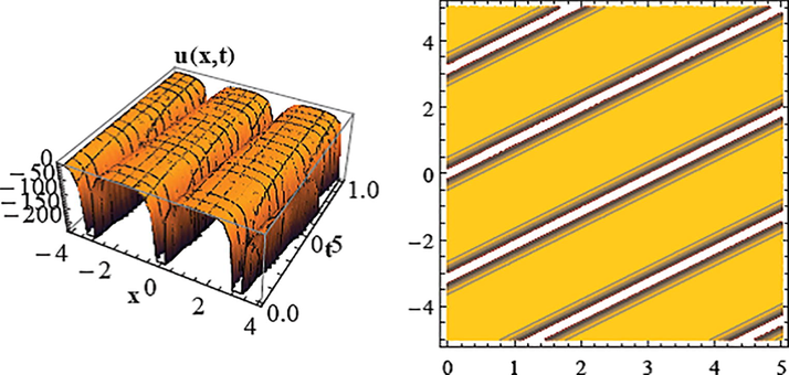
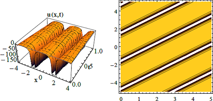
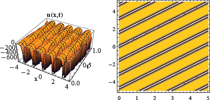
The present study effectively examines the EW and RLW equations by constructing certain periodic solitary wave solutions using the METEM. We represent the obtained solutions in three-dimensional and contour plots in Figs. 1–6 . Also, it is worth noting from Figs. 1–6 that indeed the obtained solutions are singular periodic solution.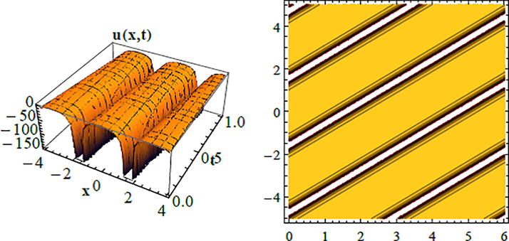

Profiles of Eq. (11) setting all parameters to unity.

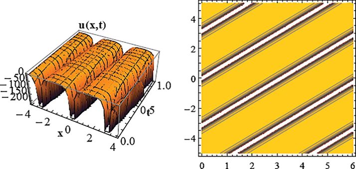
Profiles of Eq. (12) setting all parameters to unity.

Profiles of Eq. (13) setting all parameters to unity.

Profiles of Eq. (17) setting all parameters to unity.

Profiles of Eq. (18) setting all parameters to unity.

Profiles of Eq. (19) setting all parameters to unity.

However, as the main objective of the study is to analyze the effect of $U_{x}$ being the only difference between the two equations; we therefore attempt to analyze the EW equation solutions obtained in Eqs. (11)–(13) and the RLW equation solutions in Eqs. (17)–(19) which yields no clue! Thus, we resolve in studying the two-dimensional plots of both equations. We therefore conclude that the effect of $U_{x}$ is minimal and sometimes negligible when larger intervals are considered. We give below Figs. 7a and 7b. Fig. 7a gives the comparison of EW equation solution Eq. (13) and the corresponding RLW equation solution in Eq. (19); while in Fig. 7b we zoom out Fig. 7a to visualize the deeper difference. Note also that we consider Eqs. (13) and (19) for comparison plots since they both have three terms.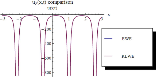

Comparing u 3 ( x , t ) of EW and RLW equations setting all parameters to unity at t = 2 .

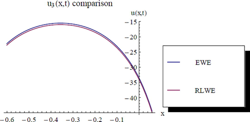
Magnification of Fig. 7a(a) with same parameters.

5 Conclusion

In conclusion, the present study analytically studies the Equal Width (EW) and Regularized Long Wave (RLW) equations by constructing certain periodic solutions and critically analyze the effect of $U_{x}$ being the only difference between the two models. Explicit dispersive solitary wave solutions are presented using the modified extended tan expansion method with the help of Mathematica software. Thus, We finally conclude from the obtained results that the effect of $U_{x}$ is minimal and sometimes negligible when larger intervals are considered after studying various two-dimensional plots of both the EW and RLW equations’ solutions (see Fig. 7a and 7b).

References

Alam N., Belgacen F.B.M., . Application of Novel (G′/G) expansion method to the regularized long wave equation. Waves Wavelets Fractals. 2015;1(1)
[Google Scholar]
Evans D.J., Raslan K.R., . Solitary waves for the generalized equal width (GEW) equation. Int. J. Comp. Math.. 2005;4
[Google Scholar]
Fan E., . Extended tanh-function method and its applications to nonlinear equations. Phys. Lett. A. 2000;277:212-218.
[Google Scholar]
Fan H.L., . The classication of the single traveling wave solutions to the generalized equal width equation. Appl. Math. Comput.. 2012;219(2):748-754.
[Google Scholar]
Hamdi S., Enright W.H., Schiesser W.E., Gottlieb J.J., . Exact solutions of the generalized equal width equation. Comp. Sci. Appl.. 2003;725–734
[Google Scholar]
Helal M.A., Mehanna M.S., . A comparison between two different methods for solving KdV Burgers equation. Chaos Solitons Fract.. 2006;28(2):320-326.
[Google Scholar]
Islam M.T., Akbar M.A., Azad M.A.K., . A rational (G/G)-expansion method and its application to modified KdV-Burgers equation and the (2+1)-dimensional Boussineq equation. Nonlinear Studies 2015
[Google Scholar]
Jafari H., Kadkhoda N., Khalique C.M., . Travelling wave solutions of nonlinear evolution equations using the simplest equation method. Comput. Math. Appl.. 2012;64(6):2084-2088.
[Google Scholar]
Korkmaz, A.E., Exact solutions of space-time fractional EW and modified EW equations. arXiv: l601.01294vl [nlin.SI], (2016).
Kudryashov N.A., . One method for finding exact solutions of nonlinear differential equations. Commun. Nonlinear Sci. Numer. Simul.. 2012;17(6):2248-2253.
[Google Scholar]
Kudryashov N.A., Demina M.V., . Travelling wave solutions of the generalized nonlinear evolution equations. Appl. Math. Comput.. 2009;210(2):551-557.
[Google Scholar]
Liu H., Li J., Zhang Q., . Lie symmetry analysis and exact explicit solutions for general Burgers’ equation. J. Comput. Appl. Math.. 2009;228:1-9.
[Google Scholar]
Lu D., Seadawy A.R., Ali A., . Dispersive travelling wave solutions of the Equal-Width and Modified Equal Width equations via mathematical methods and its applications. Results Phys.. 2018;9:313-320.
[Google Scholar]
Malfliet M., . The tanh method: a tool for solving certain classes of nonlinear evolution and wave equations. J. Comput. Appl. Math.. 2004;165:529-541.
[Google Scholar]
Morrison P.J., Meiss J.D., Cary J.R., . Scattering of regularized-long-wave solitary waves. Physica D: Nonlinear Pheno.. 1984;11(3):324-336.
[Google Scholar]
Novikov S.P., Veselov A.P., . Two-dimensional Shrodinger operator: inverse scattering transform and evolutional equations. Physica D. 1986;18(1–3):267-273.
[Google Scholar]
Nuruddeen R.I., Nass A.M., . Exact solitary wave solution for the fractional and classical GEW-Burgers equations: an application of Kudryashov method. Taibah Uni. J. Sci.. 2018;12(3):309-314.
[Google Scholar]
Ramos J.I., . Solitary wave of the EW and RLW equations. Chaos, Solitons Fractals. 2007;34(5):1498-1518.
[Google Scholar]
Shukri S., Al-Khaled K., . The extended tan method for solving systems of nonlinear wave equations. App. Math. Comp.. 2010;217
[Google Scholar]
Wazwaz A.M., . Partial Differential Equations and Solitary Waves Theory. Beijing and Springer-Verlag, Berlin Heidelberg: Higher Education Press; 2009.