Intensity-duration-frequency curve derivation from different rain gauge records

1 Introduction

The accurate measurement of rainfall is very important for hydro-climatological studies, agriculture, forecast applications, and flood hazards mitigation. However, rainfall measurement is much more complicated to accomplish than is usually appreciated (Strangeways, 2010). Rainfall is conventionally measured utilizing several types of rain gauges such as the non-recording graduated cylinder gauges or the recording weighing gauges and tipping-bucket gauges.

Tipping-bucket (TB) rain gauges are the most reliable, cost-effective, and widely used tools for rainfall depth and intensity measurement (USGS, 1999). On the other hand, the accuracy of TB gauges is known to be decreasing with increasing tip frequency (Marsalek, 1981). VanWoert et al. (2005) mentioned that a large impact on the measurement of the rain gauge may occur with increasing rainfall intensity. This impact is difficult to quantify and it is generally ignored. The primary cause of this inaccuracy is that it takes a short time for the bucket to tip. During the tipping movement of the bucket, a rainwater amount is lost since it enters into the filled bucket (Devine, 2009). The extent of gauge under-catchment depends on the TB gauge specification and the magnitude of the measured rainfall intensity. The higher the rainfall intensity, the larger this gauge’s under-catchment. Several techniques have been proposed to reduce the amount of bucket under-catchment of TB gauges during heavy rainfall. Examples of these are using TB gauges that are equipped with a siphon tube, improving the design of the bucket to diminish its tilting time and using dynamic calibration in addition to the traditional static calibration of the gauge. TB gauges that are equipped with siphon mechanisms are designed to deliver a specific amount of water to each bucket and are believed to offer outstanding performance during heavy rainfall events. Examples of such items are the RIMCO, Sutron 5600–0685, and Hydrological Services TB4 rain gauges. The siphon mechanism is utilized to control the flow into the tipping buckets that may allow them to outperform typical TB gauges during high rainfall intensity conditions. Though, evidence based on real measurements quantifying the influence of tipping-bucket gauge specification on catch efficiency of the gauge is lacking. Few researchers address this important issue such as Kimball et al. (2010) and Al-Wagdany (2016). The LTH TB gauge developed by the Department of Water Resources Engineering in Lud City, Sweden is an example for gauges that has a specially designed bucket to reduce under-catchment during heavy rainfall by diminishing tilting time to ensure fast evacuation of water from the bucket (Niemczynowicz, 1986).

Dynamic calibration methods of TB gauges assume that the volume of rainwater that tips the bucket is dependent on rainfall intensity. In other words, they are based on the assumption that the relationship between rainfall rate and water amount per tipping of the bucket is non-linear. These methods try to account for the under-catchment of the bucket by calibrating the gauge while the buckets are in motion (Humphrey et al., 1997). Dynamic calibration is performed by comparing measured rain gauge rates with actual rain intensities that are computed from the defined flow rate and funnel area of the rain gauge. Although the dynamic calibration may increase the accuracy of gauge measurements, it has the disadvantage of being a labor-intensive and time-consuming process since it is conducted by supplying numerous flow rates and recording the tipping time of the bucket. According to Humphrey et al., 1997, dynamic calibration is recommended to correct rain intensities greater than 50 mm/h. The underestimation error can reach up to 29% for rain intensities more than 150 mm/h. For rainfall intensity less than 50 mm/h, the differences between measured and corrected values are insignificant. Besides, the underestimation error is found to increase with increasing rainfall rates and gauge resolution.

Values of observed depth and duration of rainfall storms are usually sensitive to the specifications of the recoding rain gauge. Hence, it may have significant effects on the computed characteristics of rainfall extremes and the design rainfall events selection from IDF curves. These curves are mathematical formulations that are commonly used in hydrology to estimate the design storm. They are utilized to estimate the rainfall intensity for a given storm duration and return period or conversely to estimate the return period for a specific rainfall event. In other words, they explain how extreme rainfall intensities vary with duration over a range of return periods (Van de Vyver, 2015). They are considered as an important procedure commonly used to perform a risk analysis of natural hazards such as floods and droughts and assessing regional flood vulnerability. IDF curves play an essential role in designing, operating, and maintaining engineering infrastructures such as urban drainage systems, culverts, and bridges. In standard hydrologic practice, IDF curves are developed from the analysis of observed point rainfall data. IDF curves revision and update are essential since they are commonly used to estimate extreme rainfall to design water resource systems. They are typically constructed from the recording rain gauge data through frequency analysis procedure utilization. However, the development of IDF curves needs short-duration precipitation data that are generally not available especially in arid areas. The most accessible rainfall data are daily rainfall totals measured by the non-recording rain gauges. Daily rainfall can be converted into shorter durations through the utilization of reduction formula or disaggregation models (Rathnam et al., 2000). Fortunately, these techniques are not needed in this study since rainfall data with very fine temporal resolution (5-min) are available for the study area.

Several researchers used the rainfall data to construct IDF curves or to investigate the temporal distribution of rainfall events in Saudi Arabia. Al-Shaikh (1985) used Gumbel distribution to develop rainfall depth–duration–frequency relationships for four regions in Saudi Arabia. IDF curves were also developed for Abha city in southern Saudi Arabia by Al-anazi and El-Sebaie (2013). Elfeki et al. (2014) used data from rainfall events to derive dimensionless design rainfall hyetograph patterns for Saudi Arabia. Regional IDF curves for the Jeddah region in western Saudi Arabia were proposed by Awadallah (2015). Al-Amri and Subyani (2017) used Gumbel and Log Pearson III distributions combined to evaluate the maximum rainfall for the various return periods in three rainfall stations in the Al-Madinah region. Recently Ewea et al. (2016) used rainfall data from recording stations in Saudi Arabia to develop IDF curves and formulas. All of these investigations used the available rainfall data and did not consider the issue of data quality and the possible effect of rainfall input errors such as the under-catchment of tipping bucket rain gauges.

It is strongly recommended to minimize and correct rainfall input errors prior to the utilization of rainfall data series for hydrological investigations. The main driver of this investigation is the necessity to better understand the issue of under-catching of tipping-bucket rain gauges, particularly in relation to the substantial inaccuracies occurrence during extreme rainfall events. Therefore, this paper aim is to identify and understand the effect of rainfall data from different rain gauges on the IDF curves computation. This understanding is required since values of rainfall intensities obtained from IDF curves are used for designing hydro-meteorological, hydro-climatological and hydraulic structures such as canals, culverts, pipes, and dams spillways.

2 Study area

Namman basin is located in Makkah region in western Saudi Arabia and it extends between latitudes of 21° 07′ and 21° 30′ N and longitudes of 40° 00′ and 40° 20′E. The total catchment area of the basin is about 650 km² and it is located within the Arabian shield which is formed mainly from Precambrian metamorphic and plutonic rocks, and quaternary deposits filling the main wadi course. The basin is mountainous and the elevation is varying within the basin from 300 m to about 2000 m above MSL. The terrain slopes down to the Red Sea coast at the western of Saudi Arabia. Fig. 1 shows the drainage area of the Namman basin and its main tributaries.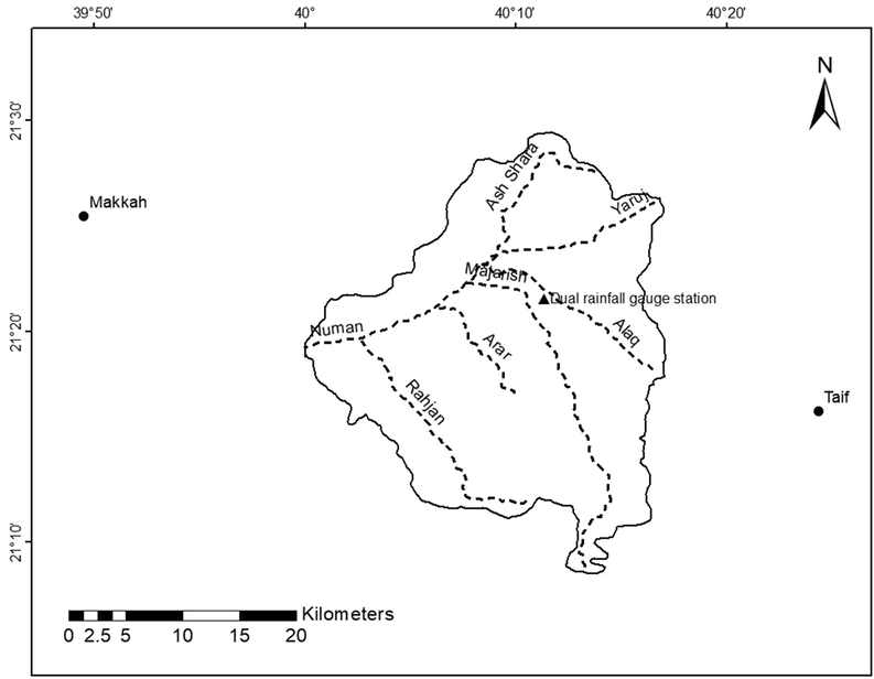

Close

Fig. 1

Location of the Dual Tipping-Bucket Rainfall Station in the Namman Basin.

Export to PPT

The location of the basin is very strategic and important since it is between two major and historic cities of the country namely, Makkah and Taif. Also, the historical groundwater galleries of Ain Zubaidah are located within the basin. These galleries were originally constructed in the midstream of the basin and they managed to provide drinking water supply to Makkah city and the surrounding holy sites for more than 1200 years. It is named after its founder Zubaidah the wife of Caliph Haroon Al-Rasheed. She noticed that there was water scarcity in Makkah and decided to establish a project that could bring the water from basins in the vicinity of Makkah to the holy sites. The project consists of a network of underground stone-lined galleries that span over a length of 27 km. Until 1974 Ain Zubaidah was able to provide over 40,000 m³/day of water. The project eventually became unable to match the increasing demand for water because the water table level declined due to excessive groundwater extraction.

The weather in the study area is affected by that zone of climate which develops in a transitional zone between the Mediterranean region and the monsoon. This climate is modified by the convectional effect of the elevated Hada Escarpments in the east and the Red Sea in the west. The temperature in the region is particularly hot during the summer season as it ranges between 33 and 49 °C. The study region is characterized by frequent rainfall events when it is compared to most other regions of Saudi Arabia. The spatial distribution of rainfall in the basin is strongly controlled by the topography and the mean annual rainfall over the basin is about 200 mm. There are two wet seasons in the area: the first starts in March and continues into May while the second extends between November and January. Rainfall data used in this study was obtained from a rainfall gauge station installed in 2006 during a research project which aimed to renovate the historical groundwater galleries of Ain Zubaidah. The location of this dual tipping-bucket rainfall station is also presented in Fig. 1.

3 Materials and method

The point precipitation data sets used in this study to derive IDF curves are obtained from the dual rainfall gauge station. This data is available for 13 years period (2006–2018) and it is unique in the region since it measures rainfall at a 5-min resolution. The two gauges are manufactured by Texas Electronics and the Hydrological Services. These gauges are henceforth referred to as TEG and HSG, respectively. The main characteristics of these TB gauges are presented in Table 1. During a rainy storm occurrence, rainfall accumulation depths are recorded at a 5-min time interval by the HSG and the TEG gauges. These values are stored in a data logger connected to these gauges that can record all rainfall events from a drizzle to a heavy rainstorm with intensities up to more than 30 mm/hour. Raw rainfall data recorded by both gauges are shown in Table 2 for the rainfall occurrence on 13/5/2017. The station provides continuous precipitation measurements for the upstream of the Namman basin since 2006. Al-Wagdany (2016) describes the rainfall station and the specifications of the two gauges.

IDF curves can be developed through frequency analysis of annual maxima rainfall data. This frequency analysis should be done following the most suitable theoretical probability function (PDF) to fit the annual extreme. Two methods can be utilized to carry out the frequency analysis. First, is utilizing the graphical procedure to estimate the exceedance probabilities from the measured precipitation data. The second is fitting theoretical PDF, which is then used to extract rainfall intensity values corresponding to a certain duration with specific exceedance probabilities.

The Gumbel Extreme Value type I PDF is the most widely used distribution for IDF analysis. This distribution which is adapted in this study can be determined as:

The process of developing the IDF curves in this investigation can be summarized in the following steps:

1. Rainfall records collection for HSG and TEG gauges.

2. Maximum rainfall depths extraction for each year and a set of different durations.

3. Mean and standard deviation calculation from maximum rainfall depths for a given duration.

4. Frequency analysis of the annual maxima rainfall records was undertaken using Gumbel Extreme Value type I PDF to calculate precipitation depths for each return period.

5. IDF curves construction from the rainfall data of the two gauges.

6. Comparing the developed IDF curves.

4 Results and discussion

Maximum annual precipitation data series are extracted from the13-year recorded data of HSG and TEG gauges for a set of durations from 5-min to 210-min. Means and standard deviations of maximum annual rainfall depth are estimated for each data set. Fig. 2 presents a comparison of annual extreme rainfall depths statistics for different durations at both gauges. The figure shows that values of maximum, mean, as well as standard deviation of the maximum rainfall series, are always higher for the HSG gauge. In addition, these values increase rapidly during the first hour of the rainstorm and become almost constant afterward. This may indicate that extreme rainstorms in the study have short durations.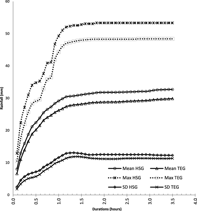

Close

Fig. 2

Comparison of Mean, Maximum, and Standard Deviation values for HSG and TEG Gauges.

Export to PPT

For each year of the available data, a comparison of annual maximum precipitation depths for various durations is presented in Table 3. The values in Table 3 were used to compute the corresponding maximum rainfall intensities as shown in Table 4. This table indicates that maximum observed values of maximum rainfall intensity were recorded in 2006 and they are associated with the 5-min maximum rainfall depths. These values are 154.8 mm/hr for HSG gauge and 126 mm/hr for the TEG gauge.

Theoretical Gumbel PDF is used to construct IDF curves for TEG and HSG gauges. Eqs. (1) and (2) as well as values of maximum rainfall statistics presented in Fig. 2 were used to compute the IDF. In Figs. 3a–3d, a comparison between developed IDF curves from precipitation records of the gauges is presented for 2, 5, 10, and 25 years return periods, respectively. These figures and Tables 3 and 4 show that the extreme rainfall depth and intensity for the HSG gauge are always higher than the corresponding values of the TEG gauge. These variations range between 8% and 21%.

Values of rainfall intensity at a specific rainfall duration are usually extracted from the IDF curves and utilized for the design of hydraulic structures used for flood protection and urban drainage systems. Therefore, it is crucial to estimate the design rainfall intensity as accurately as possible. The TEG gauge failure to provide precise rainfall depths, and hence intensities during intense storms has been observed by Al-Wagdany (2016) and Kimball et al. (2010). Al-Wagdany (2016) suggested the use of a correcting factor for TEG gauge rainfall records to increase the values by 12%.

The relationship between maximum annual rainfall depths at both gauges for different durations (5-min to 210-min) is presented in Fig. 4 in the form of a scatter plot of the maximum annual rainfall depths at the TB gauges along with the line of the best fit. This figure shows that the HSG gauge reports higher rainfall depths and hence intensities, compared to the TEG gauge. It also indicates that a strong linear correlation (R² = 0.982) exists between the maximum annual rainfall depths of the TB gauges (HSG and TEG). The linear regression line in Fig. 2 is described by the following expression:

The coefficient in 1.1 is in-line with the values that were found by Al-Wagdany (2016) and Kimball et al. (2010) for similar tipping bucket rain gauges. Therefore, Eq. (3) is used to adjust the maximum annual rainfall amounts at the TEG gauge for each duration for the period 2006–2018. The corrected values are used to compute rainfall intensities corresponding to the different durations and return periods using the Gumbel PDF.

Figs. 3a–3d present a comparison between IDF curves derived from the corrected data of the TEG gauge and the observed data from the gauge. It can be noticed from the figures that both IDF curves are very comparable. However, TEG gauge tends to underestimate rainfall intensity values particularly for very short rainfall durations (5-min and 10-min). Consequently, the application of the correcting factor to the TEG rainfall data may provide more reliable rainfall intensity values corresponding to the different rainfall durations.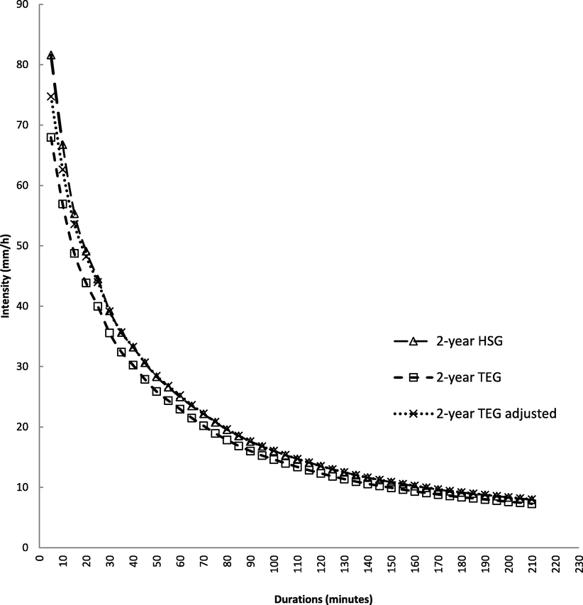

Close

Fig. 3a

IDF Curves for HSG and TEG Gauges for a 2-year return period.

Export to PPT

Close

Fig. 3b

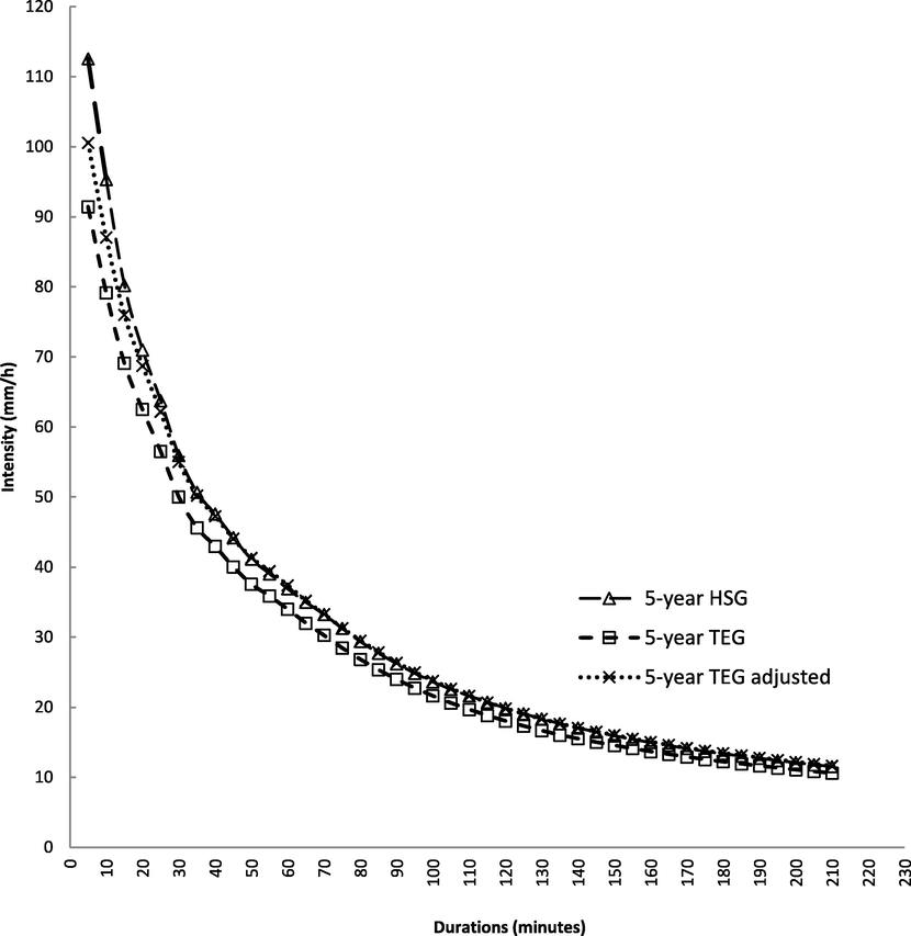
IDF Curves for HSG and TEG Gauges for a 5-year return period.

Export to PPT

Close

Fig. 3c

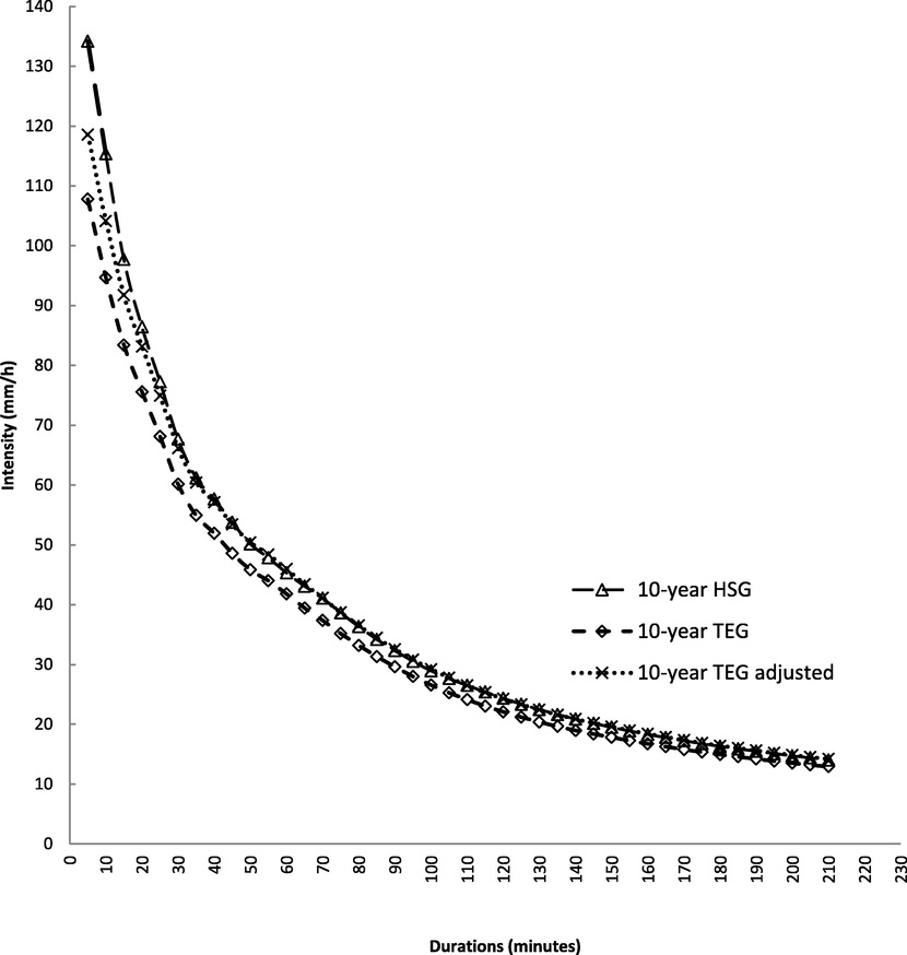
IDF Curves for HSG and TEG Gauges for a 10-year return period.

Export to PPT

Close

Fig. 3d

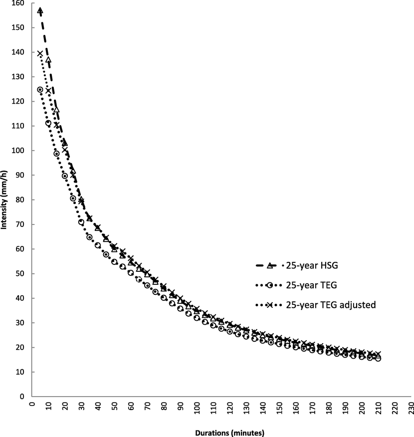
IDF Curves for HSG and TEG Gauges for a 25-year return period.

Export to PPT

Close

Fig. 4

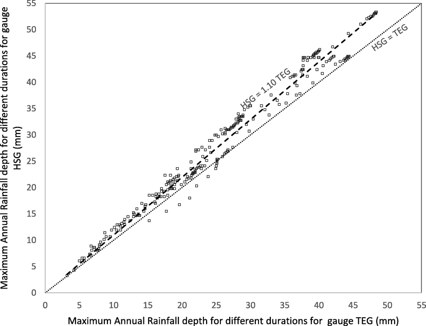
Scatter plot with linear regression of maximum annual rainfall depth from HSG Gauge versus TEG Gauge.

Export to PPT

As with any frequency analysis investigations, uncertainties in collected data and the implemented methods exist. These uncertainties can be due to gauge specifications such as شس mechanism of the tipping bucket, the effect of the siphon mechanism, and the type of gauge calibration. Other sources of uncertainties are related to the implemented methods such as the frequency analysis of the data. One of the known drawbacks of the TB gauges is that they count the number of the tippings during a chosen time interval and compute the rainfall depth by multiplying the number of tips by the volume of the bucket. Regardless of the chosen temporal resolution at which to collect the data, an amount of the rainfall will always remain in the bucket until the next rainfall period. Therefore, at the start of each rainfall event, the initial degree of bucket filling is indefinite and the bucket of the gauge can be partially filled. However, for each of the recording periods, it is expected that the remaining amount of water from the previous period will be added to the depth of the current period. Similarly, at the end of the current period, another amount of water will remain in the bucket after the last tip and it will not be considered as part of the current record. These two quantities are expected in most of the cases to cancel each other or to diminish this error in the recorded rainfall events. As stated above, this is a well-known character of tipping bucket gauges, but they are still the most accurate and widely recommended tools for measurements of rainfall events. Moreover, the static calibration of the gauge is expected to account for this systematic error of the gauge (Vasvári, 2005).

The current study shows that different types of tipping-bucket rain gauges can provide significantly different values during very intense rainfall events. This can be attributed to the gauge specifications and its ability to reduce the under-catchment amount during very intense rainfall storms. Several factors can contribute to the ability of a certain gauge to perform better concerning the amount of under-catchment. As mentioned above, the three main factors are the existence of the siphon mechanism, dynamic calibration of the gauge, and the effect of gauge resolution. Niemczynowicz, 1986, conducted a comprehensive study of dynamic calibration of three types of TB rain gauges namely, LTH gauge, PLUMATIC gauge, and RIMCO gauge. The total number of the tested gauges in the study was 26 gauges (12 LTH, 12 PLUMATIC, and 2 RIMCO). The RIMCO and PLUMTIC gauges have a similar gauge resolution of 0.20 mm while the LTH gauge has a 0.035 mm resolution. The RIMCo gauge is equipped with a siphon mechanism. The output of this study shows that the degree of non-linearity differs significantly between various types of gauges. PLUMATIC gauges were found to have the highest error of all the investigated gauges. The comparison of rainfall intensities computed using static and dynamic calibration shows that the LTH gauges also produced significant errors. The RIMCO gauges equipped with the siphon mechanism show slight non-linearity in the dynamic calibration function. The study concludes that the siphon arrangement that ensures the supply of a constant water amount to the bucket of the gauge is very effective in reducing the RIMCO gauge under-catchment effect. The values of the error in rainfall intensity measurements are very small for the RIMCO gauges. This conclusion supports the finding of the current study in which rainfall intensities of the siphon-equipped gauge (HSG) is higher than the TEG gauge. The conclusion may also indicate that the effect of gauge resolution on the values of the measured rainfall intensity can be minimized if the gauge is equipped with the siphon mechanism. The performance of RIMCO and PLUMTIC gauges was found different although the two gauges have the same value of the gauge resolution. Moreover, The LITH gauge has a very small gauge resolution (0.035 mm) and produces less error compared with the PLUMATIC gauges that have a higher gauge resolution of 0.20 mm.

Another source of uncertainty could be the impact of climate change on rainfall frequency. The IDF curves are based on the assumption that rainfall characteristics in the study region are stationary throughout the lifespan of the infrastructures (Tfwala et al., 2017). According to Fadhel et al. (2017), an upward trend in the maximum daily and short duration rainfall amounts has been observed in several regions worldwide. Some studies observed the existence of change in the frequency of rainfall exceedance overtime in the rainfall records (Bonnin, et al., 2011). For example, Mason et al. (1999) concluded that there was an increase in the intensity of extreme rainfall in South Africa between 1961 and 1990 compared to the period between 1931 and 1960. Climate change can affect the temporal and spatial variability of rainfall patterns. These changes could invalidate the assumptions on which IDF curves are based and lead to imprecise development of IDF curves.

The results of the study could also be affected by the type of the extreme-value PDF used to carry out the frequency analysis of the rainfall data. The current study utilizes the Gumbel Extreme Value type I PDF since it is the most widely used distribution for IDF analysis in arid regions. The length of the record is another factor that plays an important role in frequency analysis investigations. Viessman and Lewis (2003) stated that in performing frequency analyses on historical data at least 10 years of record should be used. Chow et al. (1989) suggested using the annual exceedance series of the data when the length of the data is less than 20 years. It should be highlighted that the purpose of this study is not to develop IDF curves that will be implemented for designing the hydraulic structures in the study area; rather is to compare IDF curves developed by utilizing the annual maximum series obtained from two different gauges. Therefore, the length of the records of 13 years should be sufficient to achieve the objective of this study. For the best of the author's knowledge, this is the only short duration rainfall data available in the country with 5 min temporal resolution. Because rainfall has high spatial variations in these areas, the comparison requires the rain gauges to be installed in the same location or at least within a very short distance from each other. Fortunately, the gauges utilized in this study are installed at the same location which is unusual, as rain gauges are normally installed far away from each other to capture the spatial variation of rainfall in the area.

Variations in the recorded rainfall amount of heavy storms among different types of gauges have significant deviations on the rainfall analysis results that utilize extreme (high intensity) rainfall values such as IDF curve extractions and design storm selection. It is recommended to investigate and compare data from different gauge types to acquire a deeper understanding of gauge type effect on intense rainfall estimation values. Another promising point of future research is to examine the influence of the dynamic calibration of TB gauges on the extraction of the IDF curves. The use of the correcting factors in the current study improves the IDF curves quality, and it is recommended to use this factor with data recorded by tipping-bucket rain gauges that are not provided with siphon mechanisms until a more in-depth investigation and comparison are conducted for different rain gauges commonly used to measure rainfall worldwide.

5 Conclusions

Tipping bucket rain gauges tend to underestimate rainfall at high intensities due to the under-catchment process associated with the tipping movement of the bucket. Understanding and quantifying rainfall under-catchment related to gauge specification are critical for design storm estimation. The most important factors that may have a major effect on reducing this under-catchment of the TB gauges are the existence of siphon mechanism, dynamic calibration of the gauge, and gauge resolution. This paper demonstrates that the measurement of extreme rainfall depths and intensities is sensitive to the specifications of the tipping-bucket gauge. Tipping-bucket rain gauges with siphon are believed to reduce the inaccuracy of rainfall measurements during heavy rainfall. This conclusion regarding the effectiveness of the siphon mechanism in reducing the amount of gauge under catchments during heavy storms is in line with the finding of Niemczynowicz (1986). The current study used fine temporal resolution precipitation records from two recording gauges (TEG and HSG) to construct the IDF curves of an important catchment in western Saudi Arabia. The under-catchment of TEG gauge during heavy storms was quantified by field observations. The HSG gauge equipped with a siphon tube reported higher values of rainfall depth and intensity compared to the TEG gauge. This may be ascribed to the siphon tube capability which permits a specific water amount to be delivered to each bucket, decreasing under-catchment all through the heavy precipitation duration (Al-Wagdany, 2016). In cases of hydrologic analysis of extreme precipitation, it is suggested to adjust the precipitation measurements of tipping-bucket gauges that are not supplied with a siphon tube. This adjustment may be performed through the utilization of a correction factor such as that suggested in this paper. However, the results presented herein offer a preliminary correction relation that needs to be tested through applications to other widely used TB gauges.

References

- Development of intensity-duration-frequency relationships for abha city in Saudi Arabia. Int. J. Comput. Eng. Res.. 2013;3(10):58-65.
- [Google Scholar]
- Generation of rainfall intensity duration frequency (IDF) curves for ungauged sites in arid region. Earth Syst. Environ.. 2017;1(8):1-12.
- Rainfall frequency studies for Saudi Arabia [M.Sc thesis]. Riyadh: Civil Engineering Department, King Saud University; 1985.
- Inconsistency in rainfall characteristics estimated from records of different rain gauges. Arab J. Geosci.. 2016;9(5):1-10.
- Regional intensity-duration-frequency curves for Jeddah region, Saudi Arabia, using ordinary and L-moments approaches. J. Flood Risk Manage.. 2015;8(3):195-207.
- Trends in rainfall exceedances in the observed record in selected areas of the United States. JAWRA J. Am. Water Resour. Assoc.. 2011;47(6):1173-1182.
- Chow, V.T., 1953. Frequency analysis of hydrologic data with special application to rainfall intensities, Bulletin no. 414, University of Illinois Eng. Expt. Station.
- Chow, V. T., Maidment D. R., Mays L. W., 1989. Applied hydrology. Water Resources Handbook; McGraw-Hill: New York, NY, USA.
- Rainfall intensity corrections with the MSC tipping bucket. CMOS Bull. SCMO. 2009;37(4):103-105.
- Development of storm hyetographs for flood forecasting in the Kingdom of Saudi Arabia. Arab J. Geosci.. 2014;7(10):4387-4398.
- Development of intensity–duration–frequency curves for the Kingdom of Saudi Arabia. Geomat. Nat. Hazards Risk. 2016;8(2):570-584.
- Uncertainty of intensity–duration–frequency (IDF) curves due to varied climate baseline periods. J. Hydrol.. 2017;547:600-612.
- A new method for automated dynamic calibration of tipping-bucket rain gauges. J. Atmos. Oceanic Technol.. 1997;14(6):1513-1519.
- The university of south alabama mesonet and coastal observing system: a technical and statistical overview. J. Atmos. Oceanic Technol.. 2010;27(9):1417-1439.
- The dynamic calibration of tipping-bucket raingauges. Nord. Hydrol.. 1986;17(3):203-214.
- Runoff Computation in a data scarce environment for urban storm water management – a case study. Proc. Congr. Int. Assoc. Hydraul. Res. 2000:446-454.
- Precipitation intensity-duration-frequency curves and their uncertainties for Ghaap plateau. Clim. Risk Manage.. 2017;16:1-9.
- Basic requirements for collecting, documenting, and reporting precipitation and stormwater-flow measurements. Open-File Report 1999:99-255.
- Bayesian estimation of rainfall intensity-duration-frequency relationships. J. Hydrol.. 2015;529:1451-1463.
- Introduction to Hydrology ((5th Edi.)). Baltimore. Maryland: Pearson Education Inc.; 2003. p. :612.
- Calibration of tipping bucket rain gauges in the Graz urban research area. Atmos. Res.. 2005;77(1–4):18-28.