

Translate this page into:
Illustration of missing data handling technique generated from hepatitis C induced hepatocellular carcinoma cohort study
⁎Corresponding author. vishwagk@rediffmail.com (Gajendra K. Vishwakarma), atanustat@gmail.com (Atanu Bhattacharjee)
-
Received: ,
Accepted: ,
This article was originally published by Elsevier and was migrated to Scientific Scholar after the change of Publisher.
Peer review under responsibility of King Saud University.
Abstract
Background and Objectives
Missing outcome data are a common occurrence for most clinical research trials. The ’complete case analysis’ is a widely adopted method to tackle with missing observations. However, it reduced the sample size of the study and thus have an impact on statistical power. Hence every effort should be made to reduce the amount of missing data. The objective of this work is to provide the application of different analytical tools to handle missing data imputation techniques through illustration.
Methods
We used Imputation techniques such as EM algorithm, MCMC, Regression, and Predictive Mean matching methods and compared the results on hepatitis C virus-induced hepatocellular carcinoma (HCV-HCC) data. The statistical models by Generalized Estimating Equations, Time-dependent Cox Regression, and Joint Modeling were applied to obtain the statistical inference on imputed data. The missing data handling technique compatible with Principle Component Analysis (PCA) was found suitable to work with high dimensional data.
Results
Joint modelling provides a slightly lower standard error than other analytical methods each imputation. Accordingly, to our methodology, Joint Modeling analysis with the EM algorithm imputation method has appeared to be the most appropriate method with HCV-HCC data. However, Generalized Estimating Equations and Time-dependent Cox Regression methods were relatively easy to run.
Conclusion
The multiple imputation methods are efficient to provide inference with missing data. It is technically robust than any ad hoc approach to working with missing data.
Keywords
EM algorithm
Regression method
Predictive mean matching
Imputation
Handling missing data

1 Introduction
Hepatocellular carcinoma (HCC) is the second leading cause of cancer-related death in sub-Saharan Africa and Asia (Bray et al., 2020). It is the sixth common cancer globally (Torre et al., 2015; European Association For The Study Of The Liver, 2012; Ferlay et al., 2015). Infection with the hepatitis C virus (HCV) found a lethal risk factor for the progression of HCC Axley et al., 2018). The risk of getting infected by HCC is 17 times more in HCV patients than in non–HCV individuals (Donato et al., 1998). It is required to have clinical trials on HCC–HCV patients to obtain better therapeutic effects. Missing data appeared in the randomized controlled trial of hepatitis C virus-induced hepatocellular carcinoma, and it is an overlooked area for robust statistical inference. It documented in a study that the HCV status was heavily missing of around 29% among the HIV infected patients (Lewden et al., 2004). It leads to a biased estimate.
Presence of missing data is acknowledged in the HCV trial (Garriga et al., 2017). Now the clinical trial, can not be performed without having repeated measurements, and repeated measurements obtained by follow-up visits raise the chance of missing data occurrence. Conventionally, the expression signature of the hepatocellular carcinoma collected with longitudinal responses for biomarkers. Commonly, each patient assigned to one of the therapy; different responses assessed at different time points. It raises the missing covariate data.
It is necessary to emphasize on a statistical methodology to impute those missing values to gather additional information from the longitudinal and survival patterns. It is common in clinical trials and may have a substantial effect on the inferences that can bedraw from the data. Understanding the cause of missing data is essential for handling the remaining data aptly. The potential reasons for missingness could be that the subjects in longitudinal studies frequently drop out before the survey get completed since they have moved out of the region, no longer get the personal benefit for participating, died, or do not like the treatment therapy. The proportion of missing observations may be huge in some studies. Reason of missingness may be due to aggressive disease and treatment toxicity. The exclusion of participants with missing measurements can have a severe impact on the study results. Measures that require painful collection procedures or confidential, invasive, time-consuming coding, and complicated laboratory analysis or compilation are more likely to be missing.
The objective of this work is to present different missing data handling techniques. The software used to achieve the objective of this work are carried out usingR CRAN ( https://cran.r-project.org/) and Statistical Analysis System (SAS).
This work is about presenting different missing data handling technique through the HCC data. Techniques like last observation carried forward (LOCF), baseline observation carried forward (BOCF), handling missing values with multivariate data analysis, the regression method, predictive mean matching, expectation–maximization (EM) algorithm, Markov chain Monte Carlo (MCMC) method, and generalized estimating equation(GEE) were presented with the illustrating data.
2 Data description
We used hepatocellular carcinoma dataset to illustrate our multiple imputation techniques-the dataset used for illustration only. Due to ethical constraints, the treatment arms were blinded. Multiple imputation techniques were compared on HCV-HCC patients data. A total of 160 patients from HCV-related HCC with liver cirrhosis and HCV-related cirrhosis without any substantial evidence of HCC were considered for analysis. The characteristics considered for the liver cirrhosis study are the Model For End-Stage Liver Disease (MELD) score[ranges from 20 to 32], age[range 30–65], Gender[Male , Female ], Alkaline Phosphate[range 62–93],SGOT[range 93–141], and SGPR[range 85–155].The MELD scores are directly proportionate to the severity of the disease. The data considered in this analysis are MELD score observed at visit 1, visit 2, visit 3, visit 4 and visit 5, respectively. The original work was published earlier (Garriga et al., 2017). The therapies were (I) ’Arm-A’ (n = 80 subjects) or (II) ’Arm-B’ (n = 80 subjects). The continuous variables were defined as age in years, Alkaline Phosphate, SGOT, SGPR, and MELD score. Subjects were followed continuously, and the death status(alive or died) were recorded. The dataset named as ”datahcv” was uploaded as supplementary file s1. The missing observations were observed from visit 2 to visit 5 for a few subjects.
3 Methodology
In this section, we will discuss the different statistical design and similar analytical tools to handle missing values. This dataset is dedicated to baseline missing data handling techniques.
In the presence of missing observations, and statistical inference requires to check, assumptions about the process that caused the missing data, which is also known as missing data mechanism. Reasons for missing data can be separated as (I) Patients lost to follow-up from the study. (II) Data entry errors. (III) Patient denial. (IV) The severely ill patient was unable to visit the clinic. (V) Faulty measurement device. (VI) Data not entered or updated, and so forth. In summary, the missing data mechanisms can be classified into three categories.
Missing data is said to be missing completely at random if the missingness does not depend on the observed or unobserved observations. The examples of this type of missing data would be data entry errors, accidental deletion of response on a questionnaire and mishandling of laboratory instrument. For example, in liver transplant study, the criteria for deciding when liver transplantation is required are mainly based on MELD. Let’s assume that the MELD score is missing for some patients. Then the missing MELD scores are MCAR if the chance of observing the missing MELD is independent of the fully observed MELD scores and the MELD that would have been seen (i.e., the disappeared MELD scores). Under MCAR, the observed data are a random sample of all the data. In such scenarios, a complete case analysis may result in more significant SEs in the model parameter estimates (i.e., loss of efficiency) in this setting. Still, no bias in the model parameter estimates is introduced when the data are MCAR. Bias is defined as the average difference between model parameter estimates and their true values (Little, 1995; Rubin, 1976).
Data are said to be missing at random (MAR) if, given the observed data, the probability of missing value does not depend on the data that are unobserved.
The missing data mechanism is said to be nonignorable or missing not at random (MNAR) if the failure to observe a value depends on the amount that would have been found or other missing values in the data set. MNAR data are most common in longitudinal studies in which missingness is the result of study dropout, toxicity, or illness.
If the technique is dependent on the missing data, and the observed data decides the outcomes, then it is classified as missing, not at random (MNAR) (Sterne et al., 2009; Dziura et al., 2013). It is not possible to differentiate the MAR and MNAR by looking at the observed data. The definition of the missing data is unknown, and it can, therefore, not be assessed if the observed data can predict the new data (Little et al., 2012; Morris et al., 2014). In this context, direct maximum likelihood method provides the unbiased estimates. However, it is not clinically suitable to assume MAR (Little et al., 2012). Further, the sensitivity analyses are required to understand the potential impact of the MNAR on the estimated results (Little et al., 2012; Morris et al., 2014). It is worth mentioning that unfortunately, one cannot determine whether missingness is MNAR or MAR solely based on the data at hand. There are different issues to handle the missing data. It is not only about understanding the type of missingness. The lost data handling technique is required to be compatible with the study design.
4 Ad hoc analysis strategy with missing data
4.1 Conventional missing value imputation strategy
The calculated mean value is defined as straightforward to replace the missing value. This is a quick step to fix the missing data problem.
Different missing data handling techniques known as the last observation carried forward (LOCF) (Laird, 1988; Roy et al., 2018) and baseline observation carried forward (BOCF) (Woolley et al., 2009). These are ad hoc imputation methods for longitudinal data. The previously observed data values as an alternative to missing data are considered. It is a procedure that the idea is to take the already found amount as a replacement for the missing data. When multiple values are missing in succession, the method searches for the last observed value.
A complete case analysis can result in biased estimates, inefficient or unrealistic standard errors. It only analyzes subjects with available data on each variable. Even though the study has simplicity, it reduces the statistical power and doesn’t use all the information. Listwise deletion and Pairwise deletion will not provide any bias in parameter estimates if the data are MCAR (Roy et al., 2018). If the data are MAR (not MCAR), then these methods will produce biased parameter estimates. Simple imputation methods such as mean imputation provide biased estimates (Woolley et al., 2009). Instead of imputing a single value for each missing value, a multiple imputation technique substitutes each missing observation.These multiply imputed data sets are then analyzed using standard statistical procedures and pooling the results from these analyses (Liu-Seifert et al., 2010; Allison, 2001).
A Model could be either the logistic or linear model decided by the type of response variable (Glasser, 1964).Thereafter, predictions for the incomplete cases are inversely calculated from the fitted model. It serves as the replacements for the missing data.
Stochastic regression is a specific step of the regression imputation technique. It used through exploring the correlation bias. The noise of the predictions is incorporated by stochastics regression modelling (Wallace et al., 2010).
4.2 Software packages for missing value imputation
The indicator method also comes with the regression method. If the covariate is missing, then each missing value can be replaced by zero and thereafter extends by the regression model with the response indicator. Separately, each incomplete observed covariate can be imputed. The ”mice’ package is useful to work on indicator method (Buuren and Groothuis-Oudshoorn, 2010).
The data set has an arbitrary missing data pattern, and it is assumed that the missing data are missing at random (MAR), that is, the probability that an observation is missing may depend on but not on . If any liver cirrhosis subject has the missing observation, the reason for this missing observation might only depend on their observed meld score observations and not on unobserved meld score observations. The purpose of this analysis was to compare the estimates from different imputation techniques namely Fully conditional specification (FCS) regression, FCS predictive mean matching, Markov chain Monte Carlo (MCMC) and expectation- maximization (EM) algorithm. The PROC MI procedure available in Statistical analysis software (SAS) was used to implement these techniques with statements such as FCS REGRESSION, FCS REGPMM, MCMC and EM with nimpute = 50. The chain = multiple had been used with method = MCMC for each imputation, and the option INITIAL = EM was used. The means and standard deviations from the available cases were the initial estimates for the EM algorithm using proc MI. The correlations are set to zero. The resulting estimates are used to initiate the MCMC process. Joint modelling, time-dependent cox model, and Generalized estimating equations were carried out to examine the predictors of death in the presence of time-dependent covariate meld score and baseline characteristics such as age, gender, Alkaline Phosphates, SGPR, and SGOT. The results of joint modelling analysis on 50 imputed datasets were combined to derive an overall effect in each imputation method: i.e., SAS procedure proc mianalyze was used to connect the parameter estimates in each imputation method. Now we illustrated different steps with multiple imputations. Especially, measures that are compatible with different study design.
4.3 Missing value imputation in high-dimensional data
Data generated with several thousands of covariates and the minimal sample size is known as high dimensional data. Generally, genomics data comes as high dimensional data. The data reduction is the main challenge for high dimensional data analysis. It is a task to reduce several thousand covariates to a minimal number of covariates. There is a different statistical technique to work with the data reduction mechanism. The widely used one is the principal component analysis(PCA). Especially continuous gene expression covariates can be reduced by PCA. The multiple correspondence analysis (MCA) reduced the categorical covariates data. Simultaneously the continuous and categorical variables are reduced by multiple factor analysis (MFA) (Lin, 2010). Suppose the number of variables are
. The parameters are contained with p variables of n individuals. The PCA helped to generate
, by specific approximation of X rank S through minimizing the least square.
. It works through singular value decomposition of X as
Conventionally, PCA is used as a data reduction technique. The only complete case analysis in possible to work with PCA. PCA works by maximizing the variance by individual-level diversity. Simultaneously, the Euclidean distance between the individual is derived. It helps to reduce the matrix size
with n individuals and p variables.
The PCA is performed by an orthogonal transformation to identify principal components. It worked by equal a linear combination of the gene expression levels and are linearly uncorrelated with each other (Roy et al., 2018). Sometimes, gene expression measurement for some individuals becomes missing. It is difficult to discard those individual’s observations due to missing information. The challenge is to have PCA compatible with missing data and perform PCA by imputing missing data. The ”missMDA” package available in R is suitable to solve the challenge. It helps to understand data visualization (Figure1). But singular value decomposition (SVD) plays a crucial role in all these data reduction techniques like PCA, MCA, and factor analysis. Now the arising of missing data are common in high dimensional data analysis. But discarding the missing data and perform analysis on complete case analysis(CCA) is the standard practice. Fortunately, the missMDA package available in the R system is useful to handle with missing data obtained from high dimensional data (Ilin and Raiko, 2010; Josse and Husson, 2016). It is compatible to work with PCA. This package imputes the missing data. Continuous, categorical, and mixed continuous and categorical can be attributed by the missMDA package. There are PCA can be performed into the imputed data. However, it is to be noted that the variance of the estimator obtained by PCA may be underestimated. The variability due to the imputation of missing values is not taken into account through this imputation. We illustrated the missMDA package application in handling missing data section in Table 2.
5 Multiple imputation
5.1 Regression method
Sometimes it gets difficult to understand about the actual probability of missing data. It requires to have missing data process for each visit by logistics regression having response variable with each data that is observed or not. Similarly, the independent variables can be linked with the missing data. The regression model works as a suitable approach in this context (Lee et al., 2018.) In this method, missing observations for each variable is imputed using the posterior predictive distribution of the parameters. Let, the continuous variable
, is the response observation of
patient with missing observations, and the model is defined as
The variable is
and the covariates are
.. The fitted model includes the regression parameter estimates
and the associated covariance matrix
, where
is the usual
inverse matrix derived from the intercept and covariates
. Where
is the estimated variance of
patient. The imputation model is defined as follows:
Where is the intercept and are regression coefficients. Multiple imputations in SAS involves three procedures. The first one is proc MI, in which the user writes the imputation model to be used and the number of imputed datasets to be produced (use FCS REG statement in proc MI and nimpute = 50). The second procedure runs the analytic model of interest (for example, proc genmod) within each of the imputed datasets. The third procedure is proc mianalyze, which pools all the estimates (coefficients and standard errors) across all the imputed datasets and produce pooled parameter estimates for the model of interest.
5.2 Predictive mean matching method
Multiple imputations is a commonly used method for handling incomplete covariates as it can provide valid inference when data are missing at random. Imputation by predictive mean matching (PMM) borrows an observed value to obtain the imputed values. It works with parametric imputation with greater robustness. It depends on being able to correctly specify the parametric model used to impute missing values, which may be difficult in many realistic settings (Morris et al., 2014). The variables with missing observations are imputed using predictive mean matching method. A linear regression model is estimated and generated a new set of coefficients randomly from the posterior predictive distribution of . Predicted observations for observed data are calculated from where as the predicted observations for unobserved data are calculated from . For each subject with a missing observation, found the closest predicted observations among the subjects with observed observation. Randomly selected one of these closest predicted observations and imputed the observed observation for the closest predicted observation. This method may be more appropriate than the regression method if there is a violation of normality assumption (Lin, 2010). In SAS, FCS REGPMM statement to be used in proc MI with nimpute = 50.
5.3 EM algorithm
The EM algorithm is an iterative procedure that finds the maximum likelihood estimate of the parameter vector by replicating the following steps: (I). The E-step calculates the conditional expectation of the complete-data log-likelihood given the observed data and the parameter estimates and (II) The M-step finds the parameter estimates to maximize the complete-data log-likelihood from the E-step (Lin, 2010; McLachlan and Krishnan, 2008). In the EM process, the observed-data log-likelihood is non-decreasing at each iteration. For multivariate normal data, suppose there are groups with distinct missing data patterns. Then the observed-data log-likelihood being maximized can be expressed as
Where, is the number of observations in the group, is a vector of observed observations corresponding to observed variables, is the corresponding mean vector, and is the associated covariance matrix.
5.4 Markov Chain Monte Carlo (MCMC) Method
The MCMC simulation shifts the computer for experimental laboratory. It helps to control various conditions to obtain the outcomes (Carsey and Harden, 2013). It documented that the MCMC simulation works as a strong tool to perform statistical methods under different setting with violated assumptions. (Takahashi, 2017). The MCMC method is used to create pseudo random draws from multidimensional data and or else intractable probability distributions through Markov chains. Suppose the data follows the multivariate normal distribution, data augmentation is applied to Bayesian inference with missing data by replicating the following steps: (I) The missing observations for observation j is denoted as and the variables with observed observations by , then the I-step draws observations for from a conditional distribution given . (II) The P-step simulates the posterior population mean vector and covariance matrix of the complete sample estimates. These new estimates are used in the I-step. If lack of prior information about the parameters, a non-informative prior is used. We may use other informative priors as well. In SAS, MCMC statement to be used in proc MI with nimpute = 50.
6 Analysis of imputed data
6.1 Generalized estimating equation
The repeatedly measured observations are always correlated. The generalized estimating equation(GEE) is technique to deal with correlated observations. The GEE is well developed and established statistical methodology (Zeger et al., 1988). Suppose there is a sample of
independent multivariate measurments and defined as (Halekoh et al., 2006)
Now i shows the cluster of
observations. The expectation
are linked with p-dimensional regression vector
by mean-link function (Halekoh et al., 2006)
Here,
is defined as scale parameter and
is a known variance function (Halekoh et al., 2006). Now
presented as a working correlation matrix completely described by the parameter vector
of length m. Let
The corresponding working covariance matrix of . Further, the diagonal matrix is .
It can be estimated as
as the solution of the equation
Finally, the covariance matrix can be formulated as
where
It help to solve work with correlated measurements by statistical modeling.
6.2 Time dependent cox regression
The cox model with time dependent covariates is defined as
The baseline hazard function defined as
.The measurement of covariates at time t is defined as
and regression coefficient is
. The covariates can be defined with different parts. The covariates may be time-independent or dependent. In our example, the prognostic biomarker is defined as time-dependent covariates. It is observed as a continuous variable. It is expected that the Prognostic biomarker will carry a time course trajectory over the follow-up period. The time-varying component helps to get an idea about covariates at baseline measurement. The regression parameter will change over time. The distributional assumption and test also play a crucial role to define covariates as prognostics marker or not. However, the distributional assumption may be avoided through the application of the conditional model by available information at time point
.
6.3 Joint longitudinal modeling
Time to event analysis help us to identify covariates that are predictable for death. Now survival analysis can be extended by the inclusion of time-dependent covariates. It is expected that the covariates should be error-free. It is relatively easy to promote the application of joint longitudinal and time to event data modelling in clinical research due to the recent advancement of computational flexibility. This work aims to explore the relationship between the imputed longitudinal covariates and explore their impact of death. Only the application of a longitudinal model may raise some biased outcomes. Some recent work in the modelling serves to work with multiple time-dependent covariates to the multiple-endpoint outcome (Nath et al., 2016; Bhattacharjee et al., 2018; Bhattacharjee, 2019).
6.4 Predictive mean matching method
The variables with missing observations are imputed using predictive mean matching method. A linear regression model is estimated and generated a new set of coefficients randomly from the posterior predictive distribution of . Predicted observations for observed data are calculated from whereas the predicted observations for unobserved data are calculated from . For each subject with a missing observation, found the closest predicted observations among the subjects with observed observation. Randomly selected one of these closest predicted observations and imputed the observed observation for the closest predicted observation. This method may be more appropriate than the regression method if there is a violation of normality assumption (Lin, 2010).
6.5 Markov chain monte carlo (MCMC) Method
The MCMC method is used to create pseudo random draws from multidimensional data and or else intractable probability distributions through Markov chains (Ilin and Raiko, 2010). It is assumed that the multivariate normal distribution follows for the response varable, data augmentation is applied to Bayesian inference with missing data by replicating the following steps: (I) The missing observations for observation j is denoted as and the variables with observed observations by , then the I-step draws observations for from a conditional distribution given . (II) The P-step simulates the posterior population mean vector and covariance matrix of the complete sample estimates.These new estimates are then used in the I-step. If the lack of prior information about the parameters, a non-informative prior can be used.
7 Results
Table 1 illustrates the baseline characteristics of liver cirrhosis patients. Table 2 depicts the result of Generalized Estimating Equations, Time-dependent Cox Regression, and Joint Modeling analysis for the data imputed by regression, EM Algorithm, Predictive Mean Matching, and MCMC methods. Longitudinal marker meld score is associated with increased mortality. Under regression imputation method, Odds of death is significantly higher for a unit increase in meld score for Generalized Estimating Equations [OR
CI): 1.390 (1.289, 1.500), P-value < 0.001] as well as for Joint Modeling [HR
CI): 1.100 (1.061, 1.141), P-value < 0.001]. However, Time-dependent Cox Regression [HR
CI): 1.043 (0.967, 1.125), P-value = 0.272] results were inconsistent with other methods. Under EM algorithm imputation method, Odds of death is significantly higher for a unit increase in meld score for Generalized Estimating Equations [OR
CI): 1.407 (1.306, 1.517), P-value < 0.001] as well as for Joint Modeling [HR
CI): 1.104 (1.068, 1.141), P-value < 0.001]. However, Time dependent Cox Regression [HR
CI): 1.046 (0.967, 1.131), P-value = 0.258] results were inconsistent with other methods. Under Predictive Mean Matching imputation method, Odds of death is significantly higher for a unit increase in meld score for Generalized Estimating Equations [OR
CI): 1.402 (1.303, 1.509), P-value < 0.001] as well as for Joint Modeling [HR
CI): 1.106 (1.071, 1.143), P-value < 0.001]. (see Fig 1).
Characteristics
Tumor-Cases
Disease Controls
Number of patients (n)
80
80
Sex
Male
70
Female
10
Mean age (in years)
Mean
48.63
48.61
(SD)
10.34
10.11
BMI
Mean
18.07
18.56
(SD)
(3.82)
(4.23)
Alkaline Phosphate
Mean
90.67
92.55
(SD)
(17.38)
(18.81)
SGOT
Mean
117.6
119.86
(SD)
(15.52)
(14.58)
SGPR
Mean
123.91
123.31
(SD)
(19.9)
(20.24)
Meld Score
Median
25
25
(SD)
1.8
1.55
TYPE
NAME
BMI
SGOT
SGPR
MEAN
5.02
3.00
3.93
COV
BMI
0.92
0.01
0.05
COV
SGOT
0.01
0.23
COV
SGPR
0.05
0.64
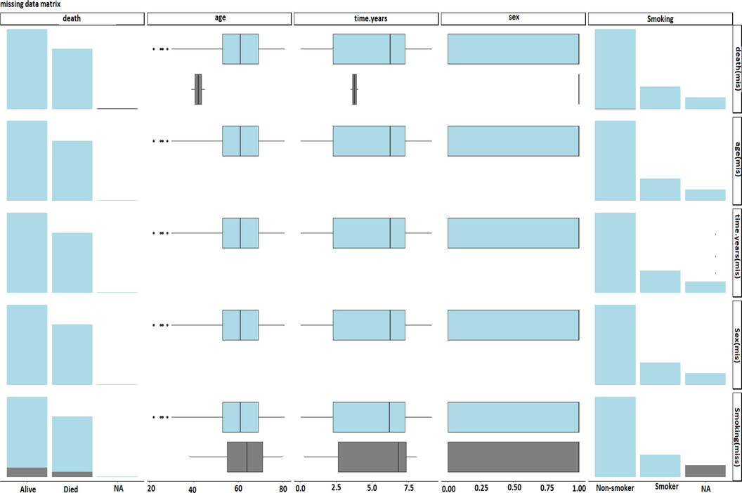
Observed and Missing data distribution comparison between died and alive patients.
However, Time dependent Cox Regression [HR CI): 1.045 (0.965, 1.132), P-value = 0.282] results were inconsistent with other methods. Under MCMC imputation method, Odds of death is significantly higher for a unit increase in meld score for Generalized Estimating Equations [OR CI): 1.401 (1.297, 1.514), P-value < 0.001] as well as for Joint Modeling [HR CI): 1.107 (1.073, 1.141), P-value < 0.001]. However, Time dependent Cox Regression [HR CI): 1.044 (0.966, 1.129), P-value = 0.273] results were inconsistent with other methods.
Table 3 represents estimates and standard error for Generalized Estimating Equations, Time-dependent cox regression, and Joint Modeling analysis for the data imputed by regression, EM Algorithm, Predictive Mean Matching, and MCMC methods. Under MCMC missing data imputation method, the estimate (Standard error) for joint modeling was 0.101(0.015) whereas estimate (Standard error) for Generalized Estimating Equation was 0.337(0.039) and estimate (Standard error) for Time-dependent cox regression was 0.043(0.039). Joint modeling gives slightly lower variation for parameter estimates as compared to other methods in all the four imputation methods. (see Table 4).
Model1
Model2
Model3
Results: Imputation Method - Regression
Variables
OR
CI)
HR
CI)
HR
CI)
Age
1.011 (0.985, 1.039)
0.986 (0.965, 1.008)
0.982 (0.960, 1.004)
Alkaline Phosphate
0.995 (0.982, 1.009)
0.995 (0.983, 1.007)
0.995 (0.983, 1.007)
Arm
0.757 (0.464, 1.237)
0.794 (0.519, 1.213)
0.804 (0.522, 1.237)
BMI
1.034 (0.971, 1.101)
0.991 (0.942, 1.042)
0.995 (0.944, 1.049)
Gender
0.606 (0.272, 1.354)
0.707 (0.373, 1.338)
0.651 (0.338, 1.253)
MELDScore
1.390 (1.289, 1.500)
1.043 (0.967, 1.125)
1.100 (1.061, 1.141)
SGOT
0.999 (0.983, 1.016)
0.988 (0.974, 1.003)
0.988 (0.974, 1.003)
SGPR
0.996 (0.983, 1.009)
1.003 (0.992, 1.014)
1.002 (0.990, 1.014)
Results: Imputation Method - Predictive Mean Matching
Variables
OR
CI)
HR
CI)
HR
CI)
Age
1.014 (0.988, 1.040)
0.987 (0.965, 1.009)
0.982 (0.961, 1.004)
Alkaline Phosphate
0.996 (0.982, 1.010)
0.995 (0.983, 1.007)
0.995 (0.983, 1.007)
Arm
0.744 (0.456, 1.214)
0.793 (0.519, 1.211)
0.818 (0.531, 1.258)
BMI
1.035 (0.972, 1.102)
0.991 (0.942, 1.043)
0.995 (0.945, 1.048)
Gender
0.570 (0.261, 1.246)
0.697 (0.367, 1.326)
0.636 (0.327, 1.239)
MELDScore
1.407 (1.306, 1.517)
1.046 (0.967, 1.131)
1.104 (1.068, 1.141)
SGOT
1.000 (0.984, 1.016)
0.988 (0.974, 1.003)
0.989 (0.974, 1.003)
SGPR
0.996 (0.983, 1.008)
1.003 (0.992, 1.014)
1.002 (0.991, 1.014)
Results: Imputation Method -EM Algorithm
Variables
OR
CI)
HR
CI)
HR
CI)
Age
1.009 (0.983, 1.035)
0.986 (0.964, 1.007)
0.980 (0.959, 1.001)
Alkaline Phosphate
0.996 (0.982, 1.010)
0.995 (0.983, 1.007)
0.995 (0.983, 1.007)
Arm
0.752 (0.459, 1.231)
0.795 (0.520, 1.215)
0.821 (0.536, 1.256)
BMI
1.030 (0.968, 1.097)
0.990 (0.942, 1.042)
0.995 (0.945, 1.048)
Gender
0.629 (0.289, 1.370)
0.714 (0.380, 1.344)
0.656 (0.346, 1.240)
MELDScore
1.402 (1.303, 1.509)
1.045 (0.965, 1.132)
1.106 (1.071, 1.143)
SGOT
0.999 (0.983, 1.015)
0.988 (0.974, 1.003)
0.988 (0.974, 1.002)
SGPR
0.997 (0.984, 1.010)
1.003 (0.992, 1.014)
1.003 (0.991, 1.014)
Results: Imputation Method -MCMC
Variables
OR
CI)
HR
CI)
HR
CI)
Age
1.012 (0.987, 1.039)
0.987 (0.965, 1.008)
0.982 (0.960, 1.003)
Alkaline Phosphate
0.995 (0.981, 1.010)
0.995 (0.983, 1.007)
0.995 (0.984, 1.007)
Arm
0.757 (0.462, 1.240)
0.794 (0.520, 1.214)
0.815 (0.532, 1.247)
BMI
1.035 (0.971, 1.102)
0.991 (0.942, 1.043)
0.997 (0.947, 1.050)
Gender
0.572 (0.263, 1.244)
0.698 (0.367, 1.326)
0.639 (0.329, 1.240)
MELDScore
1.401 (1.297, 1.514)
1.044 (0.966, 1.129)
1.107 (1.073, 1.141)
SGOT
1.000 (0.983, 1.016)
0.988 (0.974, 1.003)
0.988 (0.974, 1.003)
SGPR
0.995 (0.982, 1.008)
1.003 (0.992, 1.014)
1.003 (0.992, 1.015)
Estimate
Estimate
Estimate
Estimate
(Standard
(Standard
(Standard
(Standard
Error)
Error)
Error)
Error)
Model:Joint Modeling
Variables
Regression
Predictive Mean Matching
EM Algorithm
MCMC
Age
−0.018(0.011)
−0.020(0.011)
−0.017(0.011)
−0.018(0.011)
APhosphate
−0.005(0.006)
−0.004(0.006)
−0.004(0.006)
−0.004(0.006)
Arm
−0.218(0.219)
−0.197(0.217)
−0.201(0.219)
−0.205(0.217)
BMI
−0.004(0.026)
−0.005(0.026)
−0.004(0.026)
−0.003(0.026)
Gender
−0.429(0.334)
−0.422(0.325)
−0.451(0.339)
−0.447(0.338)
MELDScore
0.095(0.018)
0.101(0.016)
0.098(0.016)
0.101(0.015)
SGOT
−0.011(0.007)
−0.012(0.007)
−0.011(0.007)
-0.011(0.007)
SGPR
0.002(0.006)
0.002(0.005)
0.002(0.005)
0.003(0.005)
Model:Generalized Estimating Equations
Variables
Regression
Predictive Mean Matching
EM Algorithm
MCMC
Age
0.011 (0.013)
0.008(0.013)
0.013(0.013)
0.012(0.013)
AAPhosphate
−0.004(0.007)
−0.004(0.007)
−0.004(0.007)
−0.004(0.007)
Arm
−0.277(0.250)
−0.285(0.251)
−0.295(0.249)
−0.278(0.251)
BMI
0.033(0.031)
0.029(0.031)
0.034(0.032)
0.034(0.032)
Gender
−0.500(0.409)
−0.463(0.396)
−0.561(0.398)
−0.559 (0.396)
MELDScore
0.329(0.038)
0.338(0.037)
0.341(0.038)
0.337(0.039)
SGOT
−0.000(0.008)
−0.001(0.008)
−0.000(0.008)
−0.000(0.008)
SGPR
−0.004(0.006)
−0.003(0.006)
−0.004(0.006)
−0.004(0.006)
Model:Time dependent Cox Regression
Variables
Regression
Predictive Mean Matching
EM Algorithm
MCMC
Age
−0.013 (0.011)
−0.014(0.011)
−0.013(0.011)
−0.013(0.011)
AAPhosphate
−0.005(0.006)
−0.005(0.006)
−0.005(0.006)
-0.005(0.006)
Arm
−0.231 (0.216)
−0.229(0.216)
−0.232(0.216)
−0.230(0.216)
BMI
−0.009 (0.025)
−0.009(0.025)
−0.008(0.025)
−0.008(0.025)
Gender
−0.346(0.325)
−0.336(0.322)
−0.360(0.327)
−0.359(0.327)
MELDScore
0.042(0.038)
0.043(0.040)
0.045(0.039)
0.043(0.039)
SGOT
−0.011(0.007)
−0.011(0.007)
−0.011(0.007)
−0.011(0.007)
SGPR
0.003(0.005)
0.003(0.005)
0.003(0.005)
0.003(0.005)
8 Discussion
The selection of appropriate missing data techniques has a considerable impact on the clinical interpretation of the associated statistical analysis. Single imputation is a method in which missing observations are replaced by a unique representation; it may end up with underestimation of the variability and hence overestimation of test statistics. Multiple imputations impute the missing values several times, which accounts for the uncertainty and series of considerations that the correct representation could have taken. Joint modelling of longitudinal and survival data with missing covariates can not be ignored. It is tedious to work with missing observations. The presence of missing data makes it challenging to analyze, and it generated with biased inference. Now discarding the missing values and consider only available information for analysis leads to a biased estimate. Now model combined with conventional linear mixed effect for longitudinal responses with survival outcome is a joint longitudinal survival model. It is possible to work with maximizing the likelihood method. The listwise deletion method to get the complete data is valid only under MCAR conditions, but not for MAR and MNAR situations. More specifically, when the probability of missingness is dependent on the unobserved responses and covariates, it requires special techniques to handle such scenarios. A separate modelling mechanism is necessary to postulate the cases to obtain valid inference for joint models.
Three main modelling frameworks for missing observations are (I) Pattern mixture model, (II) Shared parameter model, and (III) Selection model. However, these models do not take into account the missingness of the covariates and are mainly concerned with the response variable. We presented the application of multiple imputation techniques to obtain the missing observations. Among several algorithms, we took the support of four methods for data imputation through the EM algorithm, Regression method, and MCMC procedure. The Bayesian perspective in the form of EM algorithm for imputation has produced better estimates among those methods.
The missing data imputations are an established method for repeatedly measured data. We explored how to make imputed data and jointly approached with longitudinal and survival data. By avoiding missing data, it is possible to get a biased result and generate statistical inference. Now data visualization technique is required to understand the presence of missing data and data imputation technique requires to provide by looking at the data compatibility and study design. The core message is that a joint longitudinal and survival model can be adopted, perhaps even routinely observed with missing data.
The R package named ”missMDA” is useful to impute missing data. It is suitable for PCA and MCA. Types of variables data like categorical, mixed, and continuous can be attributed. Now through multiple imputations, it is possible to study the variability of the results in PCA with other imputation technology. There are several model selection criteria to understand the presence of nonignorable missingness. The penalized validation criterion is useful as a selection modelling approach (Nath et al., 2016). There are several statistical methods to work with missing data (Fang and Shao, 2016; Cook and Weisberg, 1982; Zhu and Lee, 2001; Verbeke et al., 2001; Jansen et al., 2003 and Millar and Stewart, 2007).
The selection of appropriate missing data techniques has a considerable impact on the clinical interpretation of the associated statistical analysis. Single imputation is a method in which missing observations are replaced by a single observation which may end up with underestimation of the variability and hence overestimation of test statistics.
Multiple imputations impute the missing observation several times, which accounts for the uncertainty and series of observations that the true observation could have taken. Besides, all four imputation methods performed well for the estimation of parameters in longitudinal analysis.
The estimates for all the four imputation methods illustrate consistent results in each statistical analysis like Generalized Estimating Equations, Time-dependent Cox Regression, and Joint Modeling. Joint modelling provides a slightly lower standard error than other statistical methods in each imputation.
EM algorithm imputation method provides a slightly lower standard error in Joint Modeling analysis. Besides, the results of imputed data using Regression and Predictive mean matching were found more similar while the results of imputed data using the EM algorithm and MCMC were found more alike in Joint Modeling.
For Time-dependent Cox Regression, results of Regression and Predictive mean matching methods were found to have a slightly lower standard error. For Generalized Estimating Equations, results of Predictive mean matching and EM algorithm methods were found to be more similar.
9 Conclusion
In this article, we present efficient ways to work with the missingness of biomarker having different multiple imputation methodology and the impact on modelling. The cost to obtain the complete data is high and complex. It is required to have a specific method to work with missing data. However, we presented handling missing data by a parametric approach.
Disclosure of any funding to study
Authors received the support from the Council of Scientific and Industrial Research, Government of India, Grant No. 25(0307)/20/EMR-II to carry out this research work.
Acknowledgments
Authors are hearty thankful to Editor-in-Chief Professor Omar AI-Dossary and three anonymous learned reviewer for their valuable comments which have made substantial improvement to bring the original manuscript to its present form. Authors are also thankful to Council of Scientific and Industrial Research, Government of India, for providing support to carry out the present research work.
Declaration of Competing Interest
The authors declare that they have no known competing financial interests or personal relationships that could have appeared to influence the work reported in this paper.
References
- Missing data. Vol 136. Thousand Oaks: Sage Publications; 2001.
- Hepatitis C virus and hepatocellular carcinoma: a narrative review. J. Clin. Transl. Hepatol.. 2018;6(1):79.
- [Google Scholar]
- A joint longitudinal and survival model for dynamic treatment regimes in Presence of Competing Risk Analysis. Clin. Epidemiol. Global Health. 2019;7(3):337-341.
- [Google Scholar]
- Bayesian state-space modeling in gene expression data analysis: An application with biomarker prediction. Math. Bisci.. 2018;305:96-101.
- [Google Scholar]
- Global cancer statistics 2018: GLOBOCAN estimates of incidence and mortality worldwide for 36 cancers in 185 countries (vol 68, pg 394, 2018) CA-A Can. J. Clin.. 2020;70(4) 3.13–313
- [Google Scholar]
- Mice: Multivariate imputation by chained equations in R. J. Stat. Software 2010:1-68.
- [Google Scholar]
- Monte Carlo simulation and resampling methods for social science. Sage 2013 Publications
- [Google Scholar]
- Cook, R. D., Weisberg, S. (1982). Residuals and influence in regression. New York: Chapman and Hall. Donato, F., Boffetta, P., Puoti, M. (1998). A meta-analysis of epidemiological studies on the combined effect of hepatitis B and C virus infections in causing hepatocellular carcinoma. International journal of cancer, 75(3), 347–354.
- A meta-analysis of epidemiological studies on the combined effect of hepatitis B and C virus infections in causing hepatocellular carcinoma. Int. J. Cancer. 1998;75(3):347-354.
- [Google Scholar]
- Strategies for dealing with missing data in clinical trials: from design to analysis. Yale J. Biol. Med.. 2013;86(3):343.
- [Google Scholar]
- EASL-EORTC clinical practice guidelines: management of hepatocellular carcinoma. J. Hepatol.. 2012;56(4):908-943.
- [Google Scholar]
- Ferlay, J., Soerjomataram, I., Dikshit, R., Eser, S., Mathers, C., Rebelo, M., Bray, F. (2015). Cancer incidence and mortality worldwide: sources, methods and major patterns in GLOBOCAN 2012. International journal of cancer, 136(5), E359-E386.
- Garriga, C., Manzanares-Laya, S., García de Olalla, P., Gorrindo, P., Lens, S., Solà, R., Gurguí, M. (2017). Evolution of acute hepatitis C virus infection in a large European city: Trends and new patterns. PloS one, 12(11), e0187893.
- Linear regression analysis with missing observations among the independent variables. J. Amer. Stat. Assoc.. 1964;59(307):834-844.
- [Google Scholar]
- The R package geepack for generalized estimating equations. J. Stat. Software. 2006;15(2):1-11.
- [Google Scholar]
- Practical approaches to principal component analysis in the presence of missing values. J. Mach. Learn. Res.. 2010;11:1957-2000.
- [Google Scholar]
- A local influence approach applied to binary data from a psychiatric study. Biometrics. 2003;59(2):410-419.
- [Google Scholar]
- missMDA: a package for handling missing values in multivariate data analysis. J. Stat. Software. 2016;70(1):1-31.
- [Google Scholar]
- A multiple imputation method based on weighted quantile regression models for longitudinal censored biomarker data with missing values at early visits. BMC Med. Res. Methodol.. 2018;18(1):8.
- [Google Scholar]
- Lewden, C., Jacqmin-Gadda, H., Vildé, J. L., Bricaire, F., Waldner-Combernoux, A., May, T., APROCO Study Group. (2004). An example of nonrandom missing data for hepatitis C virus status in a prognostic study among HIV-infected patients. HIV Clin. Trials 5(4), 224-231.
- A comparison of multiple imputation with EM algorithm and MCMC method for quality of life missing data. Q. Quant.. 2010;44(2):277-287.
- [Google Scholar]
- Little, R. J. (1995). Modeling the drop-out mechanism in repeated-measures studies. Journal of the american statistical association, 90(431), 1112-1121.
- Little, R. J., D’Agostino, R., Cohen, M. L., Dickersin, K., Emerson, S. S., Farrar, J. T., Neaton, J. D. (2012). The prevention and treatment of missing data in clinical trials. New England Journal of Medicine, 367(14), 1355-1360.
- A closer look at the baseline-observation-carried-forward (BOCF) Patient Preference Adher.. 2010;4:11.
- [Google Scholar]
- McLachlan, G. J., Krishnan, T. (2008). The EM Algorithm and Extensions, vol. 382 John Wiley and Sons. Hoboken, New Jersey.[Google Scholar].
- Assessment of locally influential observations in Bayesian models. Bayesian Anal.. 2007;2(2):365-383.
- [Google Scholar]
- Morris, Tim P and Kahan, Brennan C and White, Ian R. (2014) Choosing sensitivity analyses for randomised trials: principles.BMC medical research methodology,14(1)(11).
- Tuning multiple imputation by predictive mean matching and local residual draws. BMC Med. Res. Methodol.. 2014;14(1):75.
- [Google Scholar]
- A selection modelling approach to analysing missing data of liver Cirrhosis patients. Biometr. Lett.. 2016;53(2):83-103.
- [Google Scholar]
- Expression signature of lysosomal-associated transmembrane protein 4B in hepatitis C virus-induced hepatocellular carcinoma. Int. J. Biolog. Markers. 2018;33(3):283-292.
- [Google Scholar]
- Sterne, J. A., White, I. R., Carlin, J. B., Spratt, M., Royston, P., Kenward, M. G., Carpenter, J. R. (2009). Multiple imputation for missing data in epidemiological and clinical research: potential and pitfalls. Bmj, 338.
- Statistical inference in missing data by MCMC and non-MCMC multiple imputation algorithms: Assessing the effects of between-imputation iterations. Data Sci. J.. 2017;16
- [Google Scholar]
- Torre, L. A., Bray, F., Siegel, R. L., Ferlay, J., Lortet-Tieulent, J., Jemal, A. (2015). Global cancer statistics, 2012. CA: a cancer journal for clinicians, 65(2), 87–108.
- Sensitivity analysis for nonrandom dropout: a local influence approach. Biometrics. 2001;57(1):7-14.
- [Google Scholar]
- A stochastic multiple imputation algorithm for missing covariate data in tree-structured survival analysis. Stat. Med.. 2010;29(29):3004-3016.
- [Google Scholar]
- Last-observation-carried-forward imputation method in clinical efficacy trials: review of 352 antidepressant studies. Pharmacotherapy: The Journal of Human Pharmacology and Drug. Therapy. 2009;29(12):1408-1416.
- [Google Scholar]
- Models for longitudinal data: a generalized estimating equation approach. Biometrics 1988:1049-1060.
- [Google Scholar]


