

Translate this page into:
Identification of the unknown heat source terms in a 2D parabolic equation
-
Received: ,
Accepted: ,
This article was originally published by Elsevier and was migrated to Scientific Scholar after the change of Publisher.
Peer review under responsibility of King Saud University.
Abstract
The objective of this paper is to reconstruct the unknown time-dependent heat source terms numerically, for the first time, in a two-dimensional parabolic equation in the rectangular domain with initial and Neumann boundary conditions supplemented by the temperature data as over-determination conditions. Although, the problem is ill-posed (in the sense of Hadamard) but has a unique solution. We apply the forward time central space finite difference scheme along with the Tikhonov regularization to find a stable and accurate numerical solution. The MATLAB subroutine lsqnonlin is used to solve the resulting nonlinear minimization problem. The obtained results show that accurate and stable solutions are achieved. Computational efficiency of the method is investigated by small values of CPU-time.
Keywords
Inverse source problem
2D parabolic equation
Tikhonov regularization
Nonlinear optimization

1 Introduction
In the last few decades, inverse problems for the parabolic equation have received great interest in research (Cannon, 1968; Johansson and Lesnic, 2007a,b; Hazanee et al., 2013; Hussein et al., 2018; Erdem et al., 2013; Hasanov and Pekta, 2014; Trong et al., 2006; Wang et al., 2014; Li and Qian, 2012; Singh et al., 2019). Farcas and Lesnic (2006) used the conditions of the direct problem and over-determination while Johansson and Lesnic (2007a,b) used the standard conditions of the direct and information from one supplementary temperature measurement for investigating a space-dependent heat source term for the parabolic heat equation. Li and Qian (2012) investigated the inverse problem of determining the time-dependent heat source coefficient. Authors of Hazanee et al. (2013) studied the inverse problem of finding the timewise coefficient along with the temperature solution of heat equation from nonlocal and integral conditions while in Hazanee et al. (2015), they investigated the same with a non-classical boundary and an integral over-determination conditions. Hazanee and Lesnic (2013) investigated it with non-local boundary and over-determination conditions. Huntul et al. (2018) studied the inverse problem of identifying the time- and space-dependent terms in the heat equation. Trong et al. (2006) considered the inverse problem of determining a two-dimensional heat source to construct regularized solutions and obtained error estimation explicitly. A method of reproducing kernel Hilbert space was proposed by Wang et al. Wang et al. (2014) for the inverse problem of a two-dimensional heat source. Kulbay et al. (2016) uniquely determined the solution for heat source terms and , respectively, under some regularity assumptions of inverse problems of the variable coefficients advection–diffusion equation with type separable sources from additional time-dependent temperature measurement. Recently, Hussein et al. (2018) examined the inverse problem of identifying a multi-dimensional space-dependent heat source term from boundary data. Although, the problem was linear but ill-posed. Chen et al. (2020) established the stability of an inverse source problem. The authors of Kian and Yamamoto, 2019 considered the inverse problem of recovering the time and spacewise source terms for diffusion equation. Mierzwiczak and Kolodziej (2011) investigated an inverse problem for determining unknown right-hand side in the steady two-dimensional parabolic equation while Yang (1998) and Yang et al. (2013) investigated for finding the time- and space-dependent heat sources, respectively, from the heat flux at chosen points on the boundary and final temperature measurements. The authors of Huntul and Lesnic (2020) and Huntul (2020) studied an inverse problem to reconstruct the thermal conductivity from heat flux conditions in a two-dimensional heat equations, respectively, while in Huntul (2021), author studied it for thermal conductivity and free boundary coefficients.
The inverse problem of reconstructing an unknown time or space-dependent heat source term in the heat equation has been the point of attention of many recent studies, e.g. Wang et al. (2020), Damirchi et al. (2021), Ahmadabadi et al. (2009), Yan et al. (2009), Yang and Fu (2010) and Yang et al. (2011). In these studies, in addition to being mostly restricted to one-dimensional computations, the supplementary information required to compensate for the lack of knowledge of the space-dependent heat source is a spacewise internal measurement of the temperature or a time-average of it. In this work, we study the two-dimensional parabolic problem to recover the time-dependent heat source terms numerically, for the first time, in the prescribed domain using the initial and Neumann boundary conditions, and the additional temperature data as over-determination conditions. The problem considered in this paper has already been shown to be uniquely solvable in Pabyrivska and Pabyrivskyy (2018), but the numerical reconstruction has not been studied yet. Therefore, the preeminent goal of the present work is to undertake the numerical aspect of this problem.
The paper is structured as follows. Section 2 formulated the two-dimensional inverse time-dependent source problem for the parabolic equation. Section 3 discretized the direct problem. The minimization technique of the regularized objective function is described in Section 4. Section 5 presents the computational results. Finally, Section 6 highlights the conclusions.
2 Statement of the 2D heat source problem
In the rectangular domain
, consider the inverse problem of identifying the time-dependent heat source terms
for
in the two-dimensional parabolic equation
The uniqueness of the solution of the inverse problem (1)–(6) has been established in Pabyrivska and Pabyrivskyy, 2018 and reads as follows.
Suppose that the following conditions are fulfilled:
Then, the inverse problem (1)–(6) has a unique solution in the class for .
3 Solution of the direct problem
Now, consider the direct problem (1)–(4). When are known and is to be found. Subdivide the domain into intervals and N of equal widths , and . We denote , where , and for .
We apply the forward time central space (FTCS) FDM to solve the Eq. (1) which is conditionally stable, LeVeque, 2007. So we obtain
The initial condition (2) gives
The stability condition of the explicit expression (8) is given as (Morton and Mayers, 2005)
4 Inverse solution of the 2D heat source problem
Our aim is to obtain simultaneously stable reconstructions of the heat source terms
for
and the temperature
, satisfying Eqs. (1)–(6). The inverse problem is formulated as minimizing the regularized function
The MATLAB subroutine lsqnonlin (Mathworks, 2016) is employed to minimize the objective function (14). The inverse problem given by (1)–(6) is solved subject to both exact and noisy measurements (5) and (6). The noisy data is numerically formulated, as follows:
5 Results and discussion
The solutions for
and
are presented for analytical and perturbed (noisy) data (15). The accuracy is measured by
We take , for simplicity. The lower and upper bounds for the coefficients are taken as and , respectively.
5.1 Example 1
Consider the inverse problem (1)–(6) with unknown
, and with the input data
,
It can easily be checked that with this data, the conditions
–
of Theorem 1 are fulfilled, hence the uniqueness of the solution is guaranteed. The analytical solution is given by
First of all, the accuracy of the direct problem (1)–(4) is assessed with the data (19), when
are known and given by (22), using the FTCS-FDM described in Section 3. Table 1 demonstrates that the exact and approximate solutions for (5) and (6), which exactly is given by (20), obtained with
and
, are in excellent agreement. The exact (21) and approximate
are depicted in Fig. 1.
t
0.1
0.2
0.3
…
0.8
0.9
1
N
−12.4096
−12.4096
−12.4100
−12.8395
−12.8396
−12.8400
−13.2896
−13.2897
−13.2900
…
…
…−15.8406
−15.8405
−15.8400
−16.4108
−16.4107
−16.4100
-s17.0010
−17.0009
−17.0000
120
140
Exact
−9.4001
−9.4001
−9.4000
−9.8003
−9.8003
−9.8000
−10.2005
−10.2005
−10.2000
…
…
…−12.2016
−12.2014
−12.2000
−12.6018
−12.6015
−12.6000
−13.0020
−13.0017
−13.0000
120
140
Exact
−9.4001
−9.4001
−9.4000
−9.8003
−9.8003
−9.8000
−10.2005
−10.2005
−10.2000
…
…
…−12.2016
−12.2014
−12.2000
−12.6018
−12.6015
−12.6000
−13.0020
−13.0017
−13.0000
120
140
Exact
−6.3810
−6.3809
−6.3800
−6.7215
−6.7213
−6.7200
−7.0218
−7.0215
−7.0200
…
…
…−7.9229
−7.9225
−7.9200
−7.9831
−7.9826
−7.9800
−8.0033
−8.0028
−8.0000
120
140
Exact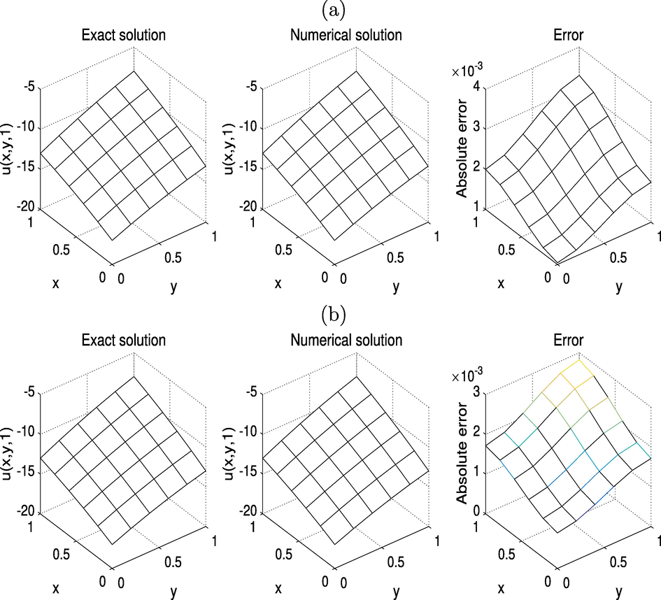
The
and absolute errors with
for: (a)
and (b)
.
In the inverse problem (1)–(6), we take the initial guesses for
and
as:
Next, we examine the inverse problem. We take a mesh size with
and
satisfying the stability condition (12). We solve the inverse problem (1)–(6) of finding the heat source terms
and
with
in
. Although not illustrated, it is reported that a rapid monotonic decreasing convergence of the objective function (14) to a very small minimum value of
is achieved in about 8 iterations. Fig. 2 depicts the obtained timewise heat source terms with
and
. An excellent agreement among the analytical (22) and computational heat sources can be noticed with
=3.3E-3,
= 8.3E−3,
= 8.3E−3 and
= 8.3E−3.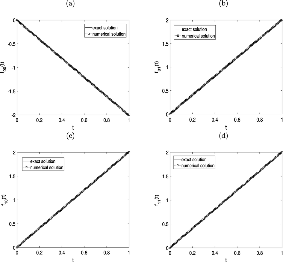
The exact (22) and numerical solutions for: (a)
, (b)
, (c)
and (d)
, with
and
, for Example 1.
Now, the stability of the computational solution is examined with respect to perturbed data. We add
noise generated by Eq. (17) to simulate the input noisy data, via Eq. (15) for
. Fig. 3 shows the objective function (14) versus the number of iterations, with
, where a monotonically decreasing convergence is obtained. The identification of the terms
is shown in Fig. 4, where the unstable (oscillation) results are obtained, if no regularization, i.e.
, is imposed with
and
, respectively. In order to stabilize these coefficients, we employ regularization with
, obtaining
. Also, from Table 2 and Fig. 4 it can be noticed that the effect of
is decreasing the unbounded behaviour (oscillatery) of the heat source terms. Therefore, the numerical results achieved with
are stable and accurate. The CPU-time is calculated to analyze the performance of the method. One can notice from Table 2 that the CPU-time is very less.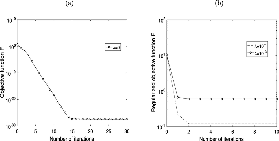
The objective function F (14) with
: (a) 0, and (b)
and
, for
, for Example 1.
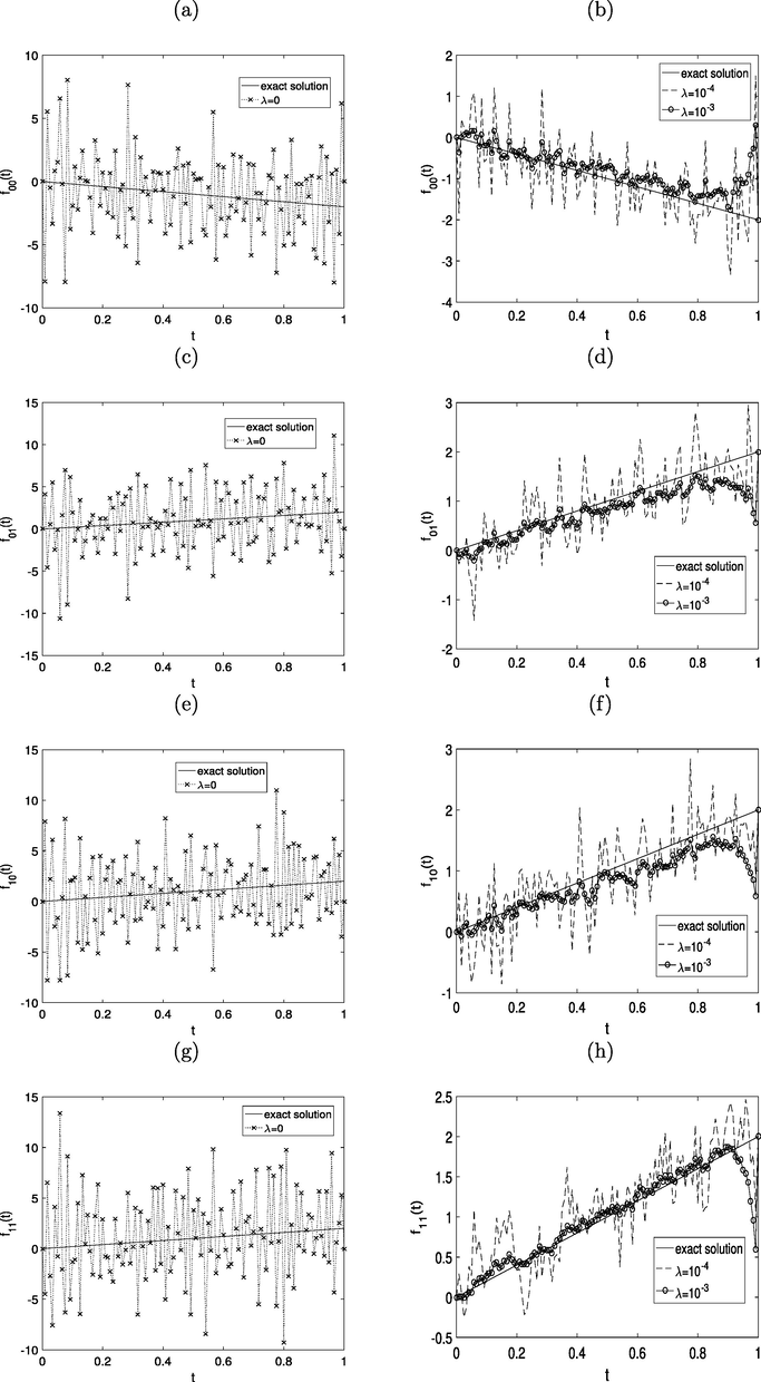
The exact (22) and numerical solutions for:
and
, with
and
, for Example 1.
p
CPU time (Mins)
0
0
3.3E−3
8.3E−3
8.3E−3
8.3E−3
3.34
0
3.1329
2.8121
1.8183
0.7362
0.4111
0.87983.5603
3.0771
1.6971
0.5410
0.3222
0.71823.6040
3.0994
1.6573
0.4929
0.3087
0.71464.2657
3.5082
1.5006
0.3672
0.1970
0.632017.23
7.01
8.11
9.21
9.45
10.49
5.2 Example 2
In Example 1, we reconstructed the smooth heat source terms
as given in (22). Now, for compliance, we examine the method to recover a nonlinear test:
Also, the conditions
–
of Theorem 1 are satisfied and therefore, the solvability of the solution is guaranteed. The analytical solution of (1)–(4) is
We take the initial guesses for
, and
as
We take and , which together with the upper bound for the source terms and satisfying the stability condition (12).
As in Example 1, first consider the case where we include no noise in
. Although not illustrated, it is reported that the F (14) decreases fastly to a low tolerance of
is reported in 17 iterations. The analytical (24) and approximate source terms
and
are plotted in Fig. 5, where the reconstructed source terms are in excellent agreement with the exact solutions.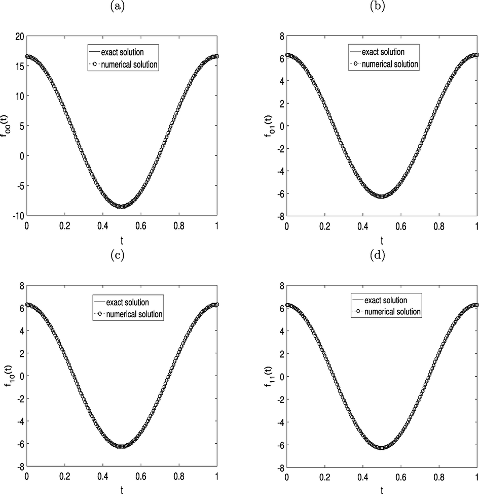
The exact (24) and numerical solutions for: (a)
, (b)
, (c)
and (d)
, with
and
, for Example 2.
Next, we include
noise in the input data
, as in (15). The corresponding exact (24) and numerical solutions for the unknown coefficients are presented in Figs. 6 and 7 for various regularizations, respectively. When
, we obtain inaccurate and unstable approximations, with RMSE values (18) of
, for
, and
, for
. We apply the Tikhonov regularization method to overcome this instability. We deduce that
for
, and
for
provides a stable and accurate numerical solutions for the unknown heat sources having the RMSE values (18) of
and
, respectively. Also, from Figs. 6, 7 and Table 3 it is observed that when p decreasing from
to
and then to zero, accuracy and stability of the approximated results increased. Finally, Figs. 6, 7 and Table 3 have the same source terms as Fig. 4 and Table 2, and we can draw the similar conclusions about the stable reconstructions for the heat source terms. It is clear from Table 3 that the CPU-time is very less.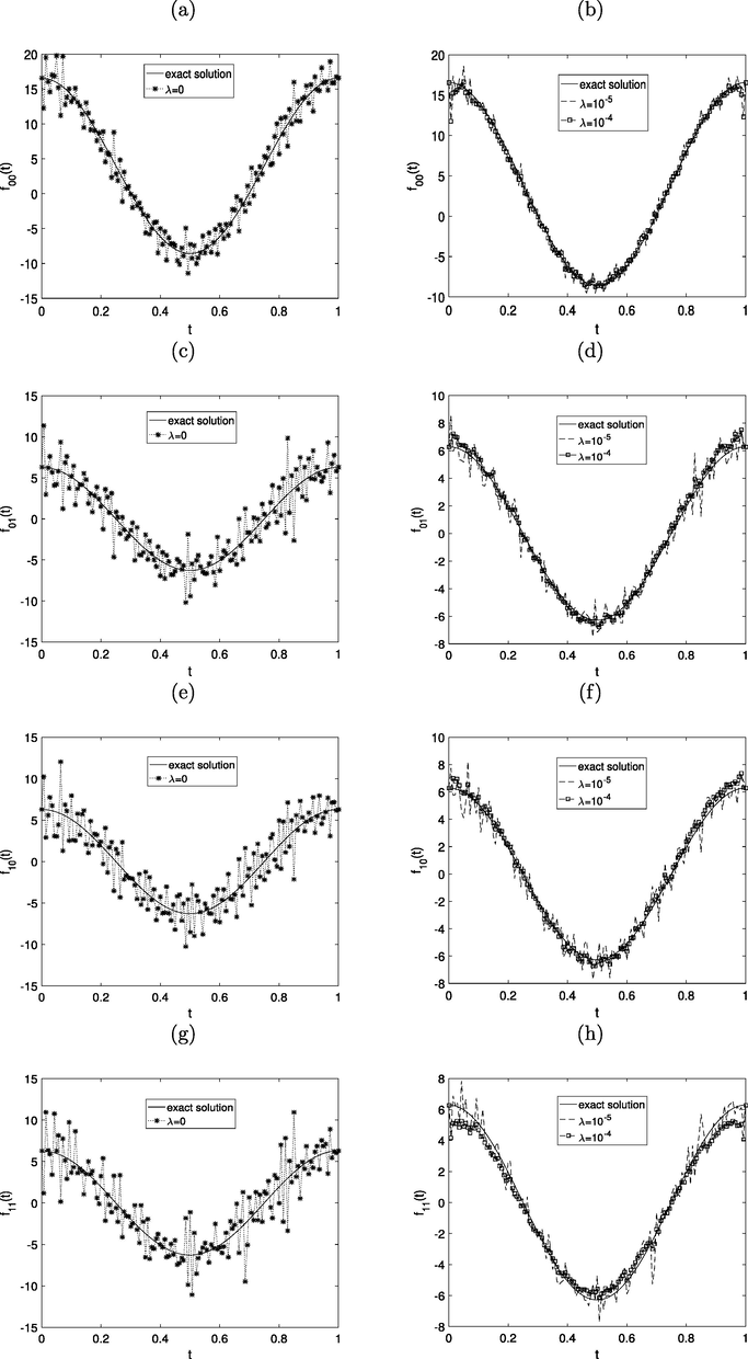
The exact (24) and numerical solutions for:
and
, with
and
, for Example 2.
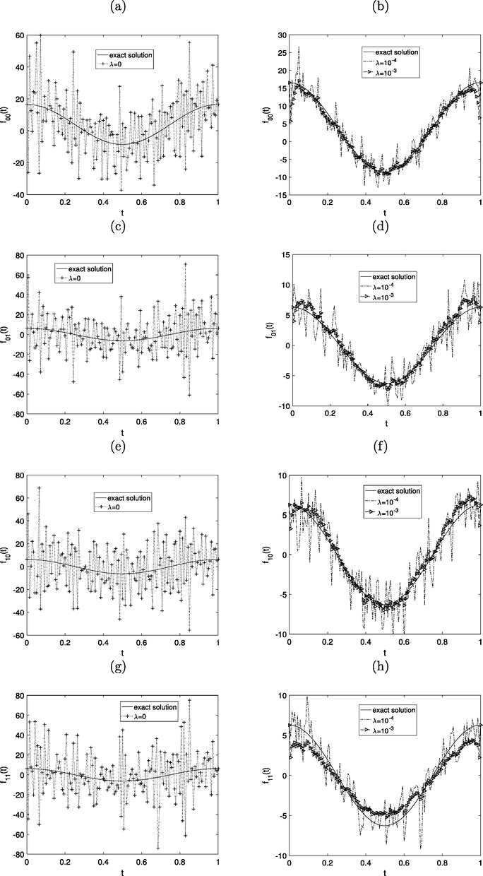
The exact (24) and numerical solutions for:
and
, with
and
, for Example 2.
p
CPU time (Mins)
0
0
8.1E−3
9.1E−3
9.1E−3
9.1E−3
4.94
0
1.6971
1.4640
0.8894
0.6815
1.63731.9709
1.6129
0.8109
0.3890
0.70382.0596
1.6946
0.8554
0.3645
0.69332.3671
1.8327
0.7671
0.5980
1.356818.26
7.81
8.37
9.28
9.54
0
16.8578
8.4550
2.9819
1.7343
3.466919.6828
7.9392
2.2630
0.8316
1.154520.5685
8.4390
2.2954
0.7640
1.170223.6539
7.4939
1.8396
1.3496
2.161529.34
13.89
14.72
15.48
16.91
6 Conclusions
The inverse problem relating to the reconstruction of the time-dependent heat source terms and the temperature in a two-dimensional parabolic equation from the over-determination conditions has been numerically studied for the first time. The direct problem has been discretized using the FTCS-FDM. The RMSE values for noise with and without regularization for Example 1 and 2 are compared. The numerical results for the inverse problem are presented and discussed. It has been concluded that for , and for provides a stable and accurate solution for the unknown heat source terms. Finally, the generalization of the proposed method to reconstruct the heat source coefficients in the three-dimensional parabolic problem is an interesting topic for future research.
Acknowledgement
The author is very thankful to the Editor in Chief and the anonymous reviewers for their valuable comments and suggestions that helped improve the paper.
Declaration of Competing Interest
The authors declare that they have no known competing financial interests or personal relationships that could have appeared to influence the work reported in this paper.
References
- The method of fundamental solutions for the inverse space-dependent heat source problem. Engineering Analysis with Boundary Elements. 2009;33:1231-1235.
- [Google Scholar]
- Determination of an unknown heat source from overspecified boundary data. SIAM Journal on Numerical Analysis. 1968;5:275-286.
- [Google Scholar]
- Conditional stability for an inverse source problem and an application to the estimation of air dose rate of radioactive substances by drone data. Mathematics in Engineering. 2020;2:26-33.
- [Google Scholar]
- Numerical approach for reconstructing an unknown source function in inverse parabolic problem. International Journal of Nonlinear Analysis and Applications. 2021;12:555-566.
- [Google Scholar]
- Identification of a spacewise dependent heat source. Applied Mathematical Modelling. 2013;37:10231-10244.
- [Google Scholar]
- The boundary-element method for the determination of a heat source dependent on one variable. Journal of Engineering Mathematics. 2006;54:375-388.
- [Google Scholar]
- A unified approach to identifying an unknown spacewise dependent source in a variable coefficient parabolic equation from final and integral overdeterminations. Applied Numerical Mathematics. 2014;78:49-67.
- [Google Scholar]
- Determination of a time-dependent heat source from nonlocal boundary conditions. Engineering Analysis with Boundary Elements. 2013;37:936-956.
- [Google Scholar]
- An inverse time-dependent source problem for the heat equation. Applied Numerical Mathematics. 2013;69:13-33.
- [Google Scholar]
- An inverse time-dependent source problem for the heat equation with a non-classical boundary condition. Applied Mathematical Modelling. 2015;39:6258-6272.
- [Google Scholar]
- Reconstruction of the timewise conductivity using a linear combination of heat flux measurements. Journal of King Saud University-Science. 2020;32:928-933.
- [Google Scholar]
- Identification of the timewise thermal conductivity in a 2D heat equation from local heat flux conditions. Inverse Problems in Science and Engineering 2020
- [CrossRef] [Google Scholar]
- Reconstructing the time-dependent thermal coefficient in 2D free boundary problems. CMC-Computers, Materials & Continua. 2021;67:3681-3699.
- [Google Scholar]
- Determination of an additive time- and space-dependent coefficient in the heat equation. International Journal of Numerical Methods for Heat and Fluid Flow. 2018;28:1352-1373.
- [Google Scholar]
- Identification of a multi-dimensional space-dependent heat source from boundary data. Applied Mathematical Modelling. 2018;54:202-220.
- [Google Scholar]
- A variational method for identifying a spacewise-dependent heat source. IMA Journal of Applied Mathematics. 2007;72:748-760.
- [Google Scholar]
- Determination of a spacewise dependent heat source. Journal of Computational and Applied Mathematics. 2007;209:66-80.
- [Google Scholar]
- Reconstruction and stable recovery of source terms and coefficients appearing in diffusion equations. Inverse Problems. 2019;35:115006
- [Google Scholar]
- Identification of separable sources for advection-diffusion equations with variable diffusion coefficient from boundary measured data. Inverse Problems in Science and Engineering. 2016;25:279-308.
- [Google Scholar]
- Numerical solution of the inverse problem of determining an unknown source term in a heat equation. Journal of Applied Mathematics. 2012;2012:1-9.
- [Google Scholar]
- Mathworks, 2016. Documentation Optimization Toolbox-Least Squares (Model Fitting) Algorithms, available at www.mathworks.com.
- The determination of heat sources in two dimensional inverse steady heat problems by means of the method of fundamental solutions. Inverse Problems in Science and Engineering. 2011;19 792–792
- [Google Scholar]
- Numerical Solution of Partial Differential Equations: An Introduction. Cambridge University Press; 2005.
- Finite Difference Methods for Ordinary and Partial Differential Equations: Steady-State and Time-Dependent Problems. Vol vol. 98. SIAM; 2007.
- Inverse problem for two-dimensional heat equation with an unknown source. In: IEEE Second International Conference on Data Stream Mining Processing (DSMP). Ukraine: Lviv; 2018. p. :361-363.
- [Google Scholar]
- Solving non-linear fractional variational problems using jacobi polynomials. Mathematics. 2019;7:224.
- [Google Scholar]
- Determination of a two-dimensional heat source: Uniqueness, regularization and error estimate. Journal of Computational and Applied Mathematics. 2006;191:50-67.
- [Google Scholar]
- Two-dimensional parabolic inverse source problem with final overdetermination in reproducing kernel space. Chinese Annals of Mathematics, Series B. 2014;35:469-482.
- [Google Scholar]
- Determination of an unknown time-dependent heat source from a nonlocal measurement by finite difference method. Acta Mathematicae Applicatae Sinica, English Series. 2020;36:151-165.
- [Google Scholar]
- Solving the two-dimensional inverse heat source problem through the linear least squares error method. International Journal of Heat and Mass Transfer. 1998;41:393-398.
- [Google Scholar]
- Inverse problem of time-dependent heat sources numerical reconstruction. Mathematics and Computers in Simulation. 2011;81:1656-1672.
- [Google Scholar]
- A simplified Tikhonov regularization method for determining the heat source. Applied Mathematical Modelling. 2010;34:3286-3299.
- [Google Scholar]
- A meshless method for solving an inverse spacewisedependent heat source problem. Journal of Computational Physics. 2009;228:123-136.
- [Google Scholar]
- Numerical identification of source terms for a two dimensional heat conduction problem in polar coordinate system. Applied Mathematical Modelling. 2013;37:939-957.
- [Google Scholar]


