Homotopy analysis method for the fractional nonlinear equations

Bahman Ghazanfari; F. Veisi

doi:10.1016/j.jksus.2010.07.019

View/Download PDF

Buy Reprints

PDF

Translate this page into:

Original Article

23 (

); 389-393

doi:

10.1016/j.jksus.2010.07.019

Homotopy analysis method for the fractional nonlinear equations

Bahman Ghazanfari^*, F. Veisi

Department of Mathematics, Faculty of Science, Lorestan University, Khoramabad 68137-17133, Iran

*Corresponding author. Mobile: +98 9161613979; fax: +98 6612218013 bahman_ghazanfari@yahoo.com (Bahman Ghazanfari)

Received: 2010-6-20, Accepted: 2010-7-18, Published: 2010-10-01

Disclaimer:
This article was originally published by Elsevier and was migrated to Scientific Scholar after the change of Publisher.

Available online 21 July 2010

Peer review under responsibility of King Saud University.

Abstract

In this paper, the homotopy analysis method is extended to investigate the numerical solutions of the fractional nonlinear wave equation. The numerical results validate the convergence and accuracy of the homotopy analysis method. Finally, the accuracy properties are demonstrated by some examples.

Keywords

Homotopy analysis method

Nonlinear differential equations

Fractional differential equations

Show Related Articles from PubMed

1 Introduction

To find the explicit solutions of nonlinear differential equations, many powerful methods have been used (Abbasbandy, 2006; He, 1998; Wazwaz, 1997; Ghasemi et al., 2007; Adomian and Adomian, 1984 ). The homotopy analysis method (HAM) (Liao, 2003, 2004; Liao and Tan, 2007; Yamashita et al., 2007 ) is a general analytic approach to get series solutions of various types of nonlinear equations. The HAM is based on homotopy, a fundamental concept in topology and differential geometry (Sen, 1983).

In recent years, considerable interest in fractional differential equations has been stimulated due to their numerous applications in the areas of physics and engineering (West et al., 2003). Many important phenomena in electromagnetics, acoustics, viscoelasticity, electrochemistry and material science are well described by differential equations of fractional order (West et al., 2003; Podlubny, 1999; Caputo, 1967 ). Though many exact solutions for linear fractional differential equation had been found, in general, there exists no method that yields an exact solution for nonlinear fractional differential equations.

2 Preliminaries and notations

In this section, let us recall the essentials of fractional calculus first. The fractional calculus is a name for the theory of integrals and derivatives of arbitrary order, which unifies and generalizes the notions of integer-order differentiation and n-fold integration. There are many books (West et al., 2003; Podlubny, 1999) that develop fractional calculus and various definitions of fractional integration and differentiation, such as Riemann–Liouville's definition, Caputo's definition and generalized function approach. For the purpose of this paper the Caputo's definition of fractional differentiation will be used, taking the advantage of Caputo's approach that the initial conditions for fractional differential equations with Caputo's derivatives take on the traditional form as for integer-order differential equations.

Definition 2.1

Caputo's definition of the fractional-order derivative is defined as

(1)

D^{α} f (t) = \frac{1}{Γ (n - α)} \int_{a}^{t} \frac{f^{(n)} (τ)}{(t - τ)^{α + 1 - n}} d τ, (n - 1 < Re (α) ⩽ n, n \in N),

where the parameter

α

is the order of the derivative and is allowed to be real or even complex, a is the initial value of function f. In this paper, only real and positive

α

will be considered. For the Caputo's derivative we have

(2)

D^{α} c = 0, (c is a constant)

(3)

D^{α} t^{β} = \{\begin{matrix} 0, & (β ⩽ α - 1), \\ \frac{Γ (β + 1)}{Γ (β - α + 1)} t^{β - α}, & (β > α - 1) \end{matrix} .

Similar to integer-order differentiation, Caputo's fractional differentiation is a linear operation: $D^{α} (λ f (t) + μ g (t)) = λ D^{α} f (t) + μ D^{α} g (t),$ where $λ, μ$ are constants, and satisfies the so-called Leibnitz rule: $D^{α} (g (t) f (t)) = \sum_{k = 0}^{\infty} (\begin{matrix} α \\ k \end{matrix}) g^{(k)} (t) D^{α - k} f (t),$ if $f (τ)$ is continuous in $[a, t]$ and $g (τ)$ has $n + 1$ continuous derivatives in $[a, t]$ .

Definition 2.2

For n to be the smallest integer that exceeds $α$ , the Caputo space-fractional derivative operator of order $α > 0$ is defined as

(4)

D_{x}^{α} u (x, t) = \frac{\partial^{α} u (x, t)}{\partial x^{α}} = \{\begin{matrix} \frac{1}{Γ (n - α)} \int_{0}^{x} (x - τ)^{n - α - 1} \frac{\partial^{n} u (τ, t)}{\partial τ^{n}} d τ, & if n - 1 < α < n, \\ \frac{\partial^{n} u (x, t)}{\partial x^{n}}, & if α = n \in N . \end{matrix}

For establishing our results, we also necessarily introduce the following Riemann–Liouville fractional integral operator.

Definition 2.3

A real function $f (x), x > 0$ , is said to be in the space $C_{μ}, μ \in R$ if there exists a real number $p (> μ)$ , such that $f (x) = x^{p} f_{1} (x)$ , where $f_{1} (x) \in C [0, \infty)$ , and it is said to be in the space $C_{μ}^{m}$ iff $f^{(m)} \in C_{μ}, m \in N$ .

Definition 2.4

The Riemann–Liouville fractional integral operator of order $α ⩾ 0$ , of a function $f \in C_{μ}, μ ⩾ - 1$ , is defined as

(5)

J^{α} f (x) = \frac{1}{Γ (α)} \int_{0}^{x} (x - t)^{α - 1} f (t) dt, α > 0, x > 0 .

Properties of the operator $J^{α}$ can be found in Podlubny (1999) and we mention only some of them in the following: For $f \in C_{μ}, μ ⩾ - 1, α, β ⩾ 0, γ ⩾ - 1$ : $\begin{matrix} J^{0} f (x) = f (x), J^{α} x^{γ} = \frac{Γ (γ + 1)}{Γ (α + γ + 1)} x^{α + γ}, \\ J^{α} J^{β} f (x) = J^{α + β} f (x), J^{α} J^{β} f (x) = J^{β} J^{α} f (x) . \end{matrix}$ Also, we need here two of its basic properties. If $m - 1 < α ⩽ m, m \in N$ and $f \in C_{μ}^{m}, μ ⩾ - 1$ , then

(6)

D^{α} J^{α} f (x) = f (x), J^{α} D^{α} f (x) = f (x) - \sum_{i = 0}^{m - 1} f^{i} (0^{+}) \frac{x^{i}}{i!}, x > 0 .

For more information on the mathematical properties of fractional derivatives and integrals, one can consult Podlubny (1999).

3 Homotopy analysis method

In this article, we apply the homotopy analysis method to the discussed problem. Let us consider the fractional differential equation:

(7)

N (u (x, t)) = 0,

where

N

is a fractional differential operator,

x

and

t

denote independent variables,

u (x, t)

is an unknown function. Liao (2003) constructed a zero-order deformation equation as follows:

(8)

(1 - q) L (ϕ (x, t; q) - u_{0} (x, t)) = q ℏ H (x, t) N (ϕ (x, t; q)),

where

ℏ \neq 0

denotes an auxiliary parameter,

H (x, t)

is an auxiliary function,

q \in [0, 1]

is an embedding parameter,

L

is an auxiliary linear operator and it possesses the property

L (C) = 0, u_{0} (x, t)

is an initial guess of

u (x, t), ϕ (x, t; q)

is a function of the homotopy-parameter

q \in [0, 1]

. It is important that one has great freedom to choose auxiliary parameter

ℏ

in homotopy analysis method. If

q = 0

and

q = 1

, it holds

(9)

ϕ (x, t; 0) = u_{0} (x, t), ϕ (x, t; 1) = u (x, t) .

Thus as q increases from 0 to 1, the solution

ϕ (x, t; q)

varies from the initial guess

u_{0} (x, t)

to the solution

u (x, t)

. Expanding

ϕ (x, t; q)

in Taylor series with respect to

q

, one has

(10)

ϕ (x, t; q) = u_{0} (x, t) + \sum_{m = 1}^{\infty} u_{m} (x, t) q^{m},

where

(11)

u_{m} (x, t) = {\frac{\partial^{m} ϕ (x, t; q)}{\partial q^{m}}|}_{q = 0} .

If the auxiliary linear operator, the initial guess, and the auxiliary parameter

ℏ

are so properly chosen, the series (10) converges at

q = 1

, one has

(12)

u (x, t) = u_{0} (x, t) + \sum_{m = 1}^{\infty} u_{m} (x, t) .

According to Eq. (11), the governing equation can be deduced from the zero-order deformation, Eq. (8). Define the vector

(13)

{\vec{u}}_{n} (x, t) = {u_{0} (x, t), u_{1} (x, t), \dots, u_{n} (x, t)} .

Differentiating Eq. (8) m times with respect to the embedding parameter q and then setting

q = 0

and finally dividing them by

m!

, we have the so-called mth-order deformation equation

(14)

L [u_{m} (x, t) - χ_{m} u_{m - 1} (x, t)] = ℏ H (x, t) R_{m} [{\vec{u}}_{m - 1} (x, t)],

where

(15)

R_{m} [{\vec{u}}_{m - 1} (x, t)] = {\frac{1}{(m - 1)!} \frac{\partial^{m - 1} N (ϕ (x, t; q))}{\partial q^{m - 1}}|}_{q = 0},

and

(16)

χ_{m} = \{\begin{matrix} 0, & m ⩽ 1, \\ 1, & m > 1 . \end{matrix}

The mth-order deformation Eq. (14) is linear and thus can be easily solved, especially by means of symbolic computation software such as MATLAB.

4 Application

Consider the following two-dimensional nonlinear differential equation of fractional order, with the indicated initial conditions:

(17)

\{\begin{matrix} \frac{\partial^{α} u}{\partial x^{α}} - u \frac{\partial^{2} u}{\partial t^{2}} = ψ (x, t), 0 ⩽ x, t ⩽ 1, 1 < α ⩽ 2 \\ u (0, t) = f (t), \frac{\partial}{\partial x} u (0, t) = g (t) . \end{matrix}

We rewrite Eq. (17) in an operator form as follows:

(18)

D_{x}^{α} u = u \frac{\partial^{2} u}{\partial t^{2}} + ψ (x, t) .

Although, we have freedom to choose an initial guess, one has

(19)

J_{x}^{α} D_{x}^{α} u = J_{x}^{α} [u \frac{\partial^{2} u}{\partial t^{2}} + ψ (x, t)],

which gives, according to Eq. (6), that

(20)

u = \sum_{k = 0}^{n - 1} u^{(k)} (0, t) \frac{x^{k}}{k!} + J_{x}^{α} [u \frac{\partial^{2} u}{\partial t^{2}} + ψ (x, t)],

where as

1 < α ⩽ 2

, so

n = 2

. Neglecting the unknown terms on the right-hand side of Eq. (20), we have the initial guess

(21)

u_{0} = f (t) + xg (t) + J_{x}^{α} [ψ (x, t)] .

Therefore Eq. (20) can be written as

(22)

u = f (t) + xg (t) + J_{x}^{α} [u \frac{\partial^{2} u}{\partial t^{2}} + ψ (x, t)] .

It is straightforward for us to choose the auxiliary linear operator

(23)

L (ϕ) = D_{x}^{α} ϕ .

For simplicity, we define, according to Eq. (18), the nonlinear operator

(24)

N (ϕ) = D_{x}^{α} ϕ - [ϕ \frac{\partial^{2} ϕ}{\partial t^{2}} + ψ (x, t)] .

According to Eqs. (14) and (23), one has

(25)

J_{x}^{α} D_{x}^{α} [u_{m} (x, t) - χ_{m} u_{m - 1} (x, t)] = ℏ J_{x}^{α} {H (x, t) R_{m} [{\vec{u}}_{m - 1} (x, t)]},

where

(26)

R_{m} [{\vec{u}}_{m - 1} (x, t)] = D_{x}^{α} u_{m - 1} - [ψ (x, t) (1 - χ_{m}) + \sum_{j = 0}^{m - 1} u_{j} \frac{\partial^{2} u_{m - 1 - j}}{\partial t^{2}}] .

Substituting Eq. (26) into Eq. (25), and choosing

H (x, t) = 1

, we find

(27)

u_{1} = - ℏ J_{x}^{α} \{u_{0} \frac{\partial^{2} u_{0}}{\partial t^{2}}\},

and for

m ⩾ 2

we have

(28)

u_{m} = (ℏ + 1) u_{m - 1} (x, t) - ℏ J_{x}^{α} \{\sum_{j = 0}^{m - 1} u_{j} \frac{\partial^{2} u_{m - 1 - j}}{\partial t^{2}}\} .

Consider the fractional nonlinear wave equation as

(29)

\{\begin{matrix} \frac{\partial^{α}}{\partial x^{α}} u - u \frac{\partial^{2}}{\partial t^{2}} u = 1 - 1 / 2 (x^{2} + t^{2}), 0 ⩽ x, t ⩽ 1, 1 < α ⩽ 2 \\ u (0, t) = \frac{t^{2}}{2}, \frac{\partial}{\partial x} u (0, t) = 0 . \end{matrix}

The exact solution for

α = 2

, is

u (x, t) = (x^{2} + t^{2}) / 2

Using Eqs. (9), (17), (27) and (28) we have

(30)

u_{0} = \frac{t^{2}}{2} + (1 - \frac{t^{2}}{2}) \frac{x^{α}}{Γ (α + 1)} - \frac{x^{2 + α}}{Γ (α + 3)},

(31)

u_{1} = - ℏ J_{x}^{α} \{u_{0} \frac{\partial^{2}}{\partial t^{2}} u_{0}\}

(32)

u_{2} = (1 + ℏ) u_{1} - ℏ J_{x}^{α} \{u_{0} \frac{\partial^{2}}{\partial t^{2}} u_{1} + u_{1} \frac{\partial^{2}}{\partial t^{2}} u_{0}\}

(33)

u_{3} = (1 + ℏ) u_{2} - ℏ J_{x}^{α} \{u_{0} \frac{\partial^{2}}{\partial t^{2}} u_{2} + u_{1} \frac{\partial^{2}}{\partial t^{2}} u_{1} + u_{2} \frac{\partial^{2}}{\partial t^{2}} u_{0}\}

⋮

Therefore, from Eq. (12), we have

(34)

u = u_{0} + u_{1} + u_{2} + \dots .

More approximation is done by MATLAB package. We first investigate the influence of the auxiliary parameter

ℏ

on the convergence of the series by plotting the so-called

ℏ

-curves for

10 th

-order approximation of Eq. (34) at

x = 0.25

and

t = 0.2

, when

α = 2

We still have freedom to choose the auxiliary parameter $ℏ$ . To investigate the influence of $ℏ$ on the solution series, we first consider the convergence of some related series such as $\partial u / \partial x, \partial^{2} u / \partial x^{2}$ , and $\partial^{3} u / \partial x^{3}$ . These curves contain a horizontal line segment. This horizontal line segment denotes the valid region of $ℏ$ which guaranteed the convergence of related series. It is observed the valid region for h is $- 3 < ℏ < 1$ as shown in Fig. 1. Thus the middle point of this interval. i.e., −1 is an appropriate selection for $ℏ$ in which the numerical solution converges (Ganjiani, 2010). For $5 th$ -order approximations and $ℏ = - 1$ , the approximate solution of u is compared with its exact solution depicted in Fig. 2 for $α = 2$ . Fig. 3 shows the HAM solution ( $α = 1.8$ ) with exact solution ( $α = 2$ ). The approximate solution for $ℏ = - 1, α = 2$ and $x = 0.25$ is completely matched with the exact solution as shown in Fig. 4.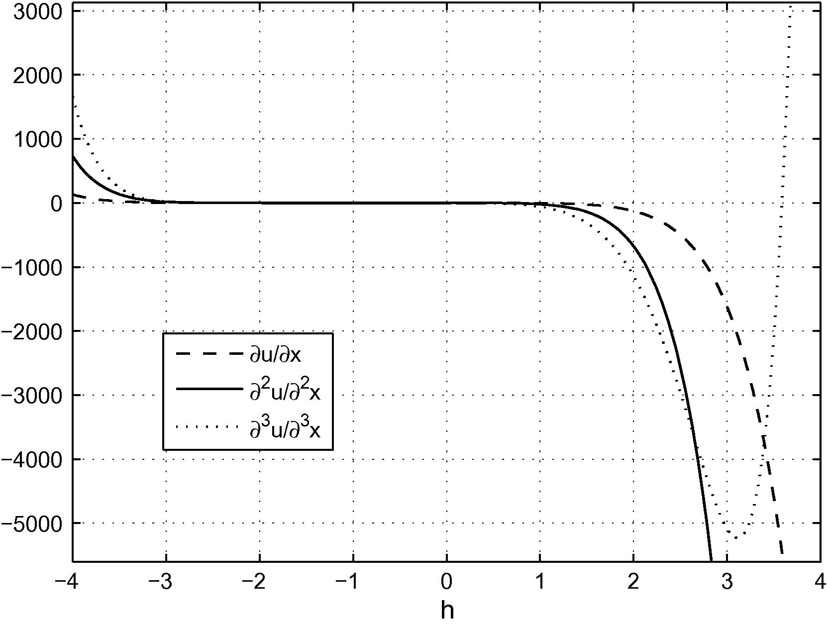

The ℏ -curves at ( x , t ) = ( 0.25 , 0.2 ) for 10 th -order approximations.

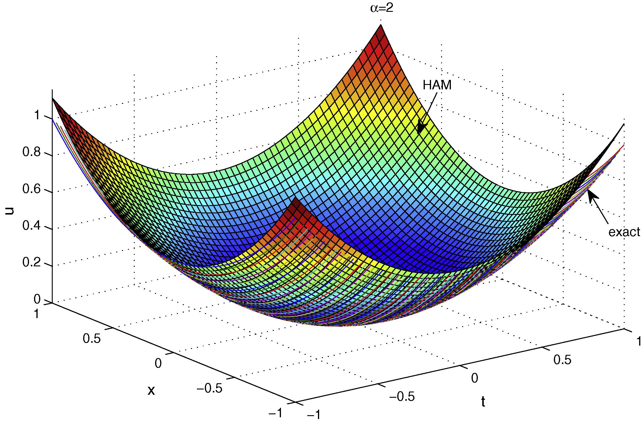
Comparison of HAM solution with the exact solution for α = 2 .

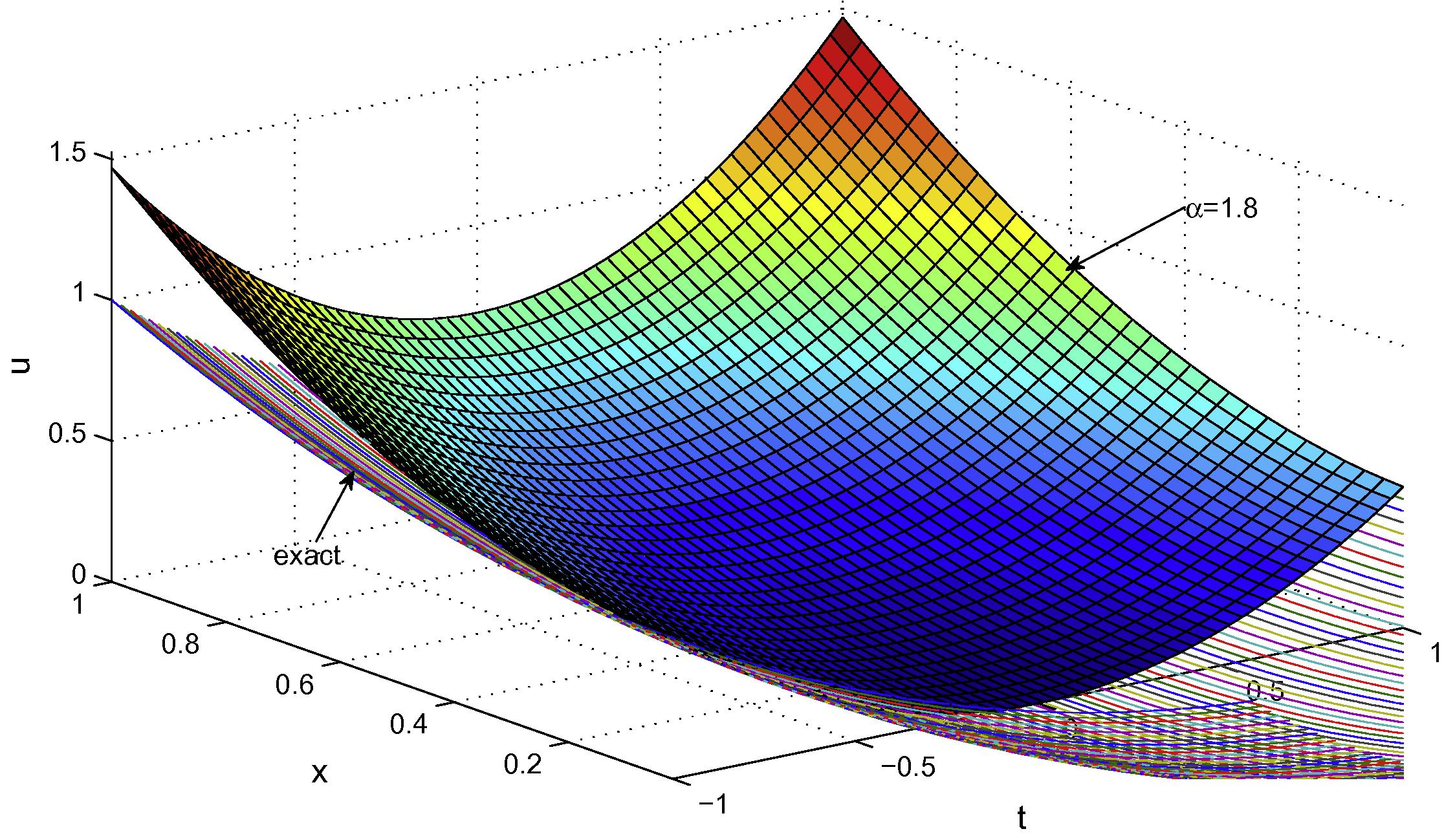
Comparison of HAM solution for α = 1.8 with the exact solution for α = 2 .

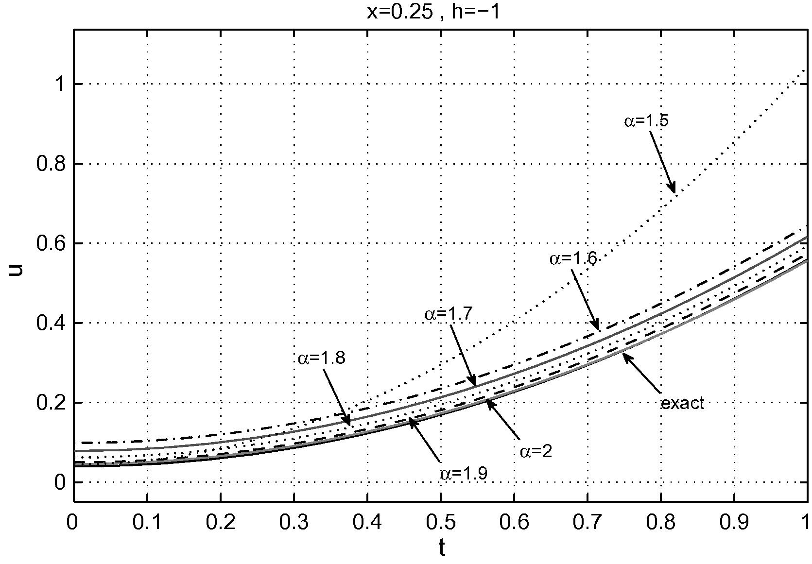
The variation of 5 th -order approximation solution of Eq. (34) with α .

5 Conclusion

In this paper, the homotopy analysis method has been applied for the numerical solutions of the fractional nonlinear wave equation. The results obtained in this work confirm the notion that the HAM is a powerful and efficient technique for finding numerical solutions for fractional nonlinear differential equations which have great significance in different fields of science and engineering.

References

Abbasbandy S., . Iterated He's homotopy perturbation method for quadratic Riccati differential equation. Appl. Math. Comput.. 2006;175:581-589.
[Google Scholar]
Adomian G., Adomian G.E., . A global method for solution of complex systems. Math. Model.. 1984;5:521-568.
[Google Scholar]
Caputo M., . Linear models of dissipation whose Q is almost frequency independent – Part II. J. R. Astron. Soc.. 1967;13:529-539.
[Google Scholar]
Ganjiani M., . Solution of nonlinear fractional differential equations using homotopy analysis method. Appl. Math. Model.. 2010;34:1634-1641.
[Google Scholar]
Ghasemi M., Tavassoli Kajani M., Davari A., . Numerical solution of two-dimensional nonlinear differential equation by homotopy perturbation method. Appl. Math. Comput.. 2007;189:341-345.
[Google Scholar]
He J.H., . An approximate solution technique depending upon an artificial parameter. Commun. Nonlinear Sci. Numer. Simul.. 1998;3(2):92-97.
[Google Scholar]
Liao S.J., . Beyond Perturbation: Introduction to the Homotopy Analysis Method. Boca Raton: Chapman & Hall/CRC Press; 2003.
Liao S.J., . On the homotopy analysis method for nonlinear problems. Appl. Math. Comput.. 2004;147:499-513.
[Google Scholar]
Liao S.J., Tan Y., . A general approach to obtain series solutions of nonlinear differential equations. Stud. Appl. Math.. 2007;119:297-355.
[Google Scholar]
Podlubny I., . Fractional Differential Equations. San Diego: Academic Press; 1999.
Sen S., . Topology and Geometry for Physicists. Florida: Academic Press; 1983.
Wazwaz A.M., . Necessary conditions for the appearance of noise terms in decomposition solution series. J. Math. Anal. Appl.. 1997;5:265-274.
[Google Scholar]
West B.J., Bolognab M., Grigolini P., . Physics of Fractal Operators. New York: Springer; 2003.
Yamashita M., Yabushita K., Tsuboi K., . An analytic solution of projectile motion with the quadratic resistance law using the homotopy analysis method. J. Phys. A. 2007;40:8403-8416.
[Google Scholar]

Introduction

Preliminaries and notations

Homotopy analysis method

Application

Conclusion

Fulltext Views
30

PDF downloads
5

View/Download PDF
Download Citations

BibTeX
RIS

Show Sections

[1] Abbasbandy S., . Iterated He's homotopy perturbation method for quadratic Riccati differential equation. Appl. Math. Comput.. 2006;175:581-589.
[Google Scholar]

[2] Adomian G., Adomian G.E., . A global method for solution of complex systems. Math. Model.. 1984;5:521-568.
[Google Scholar]

[3] Caputo M., . Linear models of dissipation whose Q is almost frequency independent – Part II. J. R. Astron. Soc.. 1967;13:529-539.
[Google Scholar]

[4] Ganjiani M., . Solution of nonlinear fractional differential equations using homotopy analysis method. Appl. Math. Model.. 2010;34:1634-1641.
[Google Scholar]

[5] Ghasemi M., Tavassoli Kajani M., Davari A., . Numerical solution of two-dimensional nonlinear differential equation by homotopy perturbation method. Appl. Math. Comput.. 2007;189:341-345.
[Google Scholar]

[6] He J.H., . An approximate solution technique depending upon an artificial parameter. Commun. Nonlinear Sci. Numer. Simul.. 1998;3(2):92-97.
[Google Scholar]

[7] Liao S.J., . Beyond Perturbation: Introduction to the Homotopy Analysis Method. Boca Raton: Chapman & Hall/CRC Press; 2003.

[8] Liao S.J., . On the homotopy analysis method for nonlinear problems. Appl. Math. Comput.. 2004;147:499-513.
[Google Scholar]

[9] Liao S.J., Tan Y., . A general approach to obtain series solutions of nonlinear differential equations. Stud. Appl. Math.. 2007;119:297-355.
[Google Scholar]

[10] Podlubny I., . Fractional Differential Equations. San Diego: Academic Press; 1999.

[11] Sen S., . Topology and Geometry for Physicists. Florida: Academic Press; 1983.

[12] Wazwaz A.M., . Necessary conditions for the appearance of noise terms in decomposition solution series. J. Math. Anal. Appl.. 1997;5:265-274.
[Google Scholar]

[13] West B.J., Bolognab M., Grigolini P., . Physics of Fractal Operators. New York: Springer; 2003.

[14] Yamashita M., Yabushita K., Tsuboi K., . An analytic solution of projectile motion with the quadratic resistance law using the homotopy analysis method. J. Phys. A. 2007;40:8403-8416.
[Google Scholar]