

Translate this page into:
Generalized non-integer Lennard-Jones potential function vs. generalized Morse potential function for calculating cohesive energy and melting point of nanoparticles
-
Received: ,
Accepted: ,
This article was originally published by Elsevier and was migrated to Scientific Scholar after the change of Publisher.
Peer review under responsibility of King Saud University.
Abstract
A generalized non-integer Lennard-Jones (L-J) potential function with an additional parameter is proposed to calculate the cohesive energy and melting point of nanoparticles. The model based on the new generalized non-integer L-J potential function has been successful in predicting experimental values. The calculated cohesive energies show an excellent agreement with the experimental values of the cohesive energies of molybdenum (Mo) and tungsten (W) nanoparticles (Kim et al., 2002). Moreover, the calculated melting points based on the generalized non-integer L-J potential function agree with the experimental values for large gold (Au) nanoparticles including atoms (Buffat and Borel, 1976) and small silica-encapsulated gold (Au) nanoparticles including atoms (Dick et al., 2002). The stability of nanoparticles is due to two conditions: the increase of the range of the attractive force and the high gradient attractive interaction in the potential function when .
Keywords
Lennard-Jones potential function, Morse potential function
Cohesive energy
Melting point
Nanoparticles

1 Introduction:
The size dependence of the physical properties of nanoparticles is one of the most important research topics which relates to the cohesive energy of nanoparticles (Qi, 2016). Many theoretical models were produced such as the surface-to-volume atomic ratio (Xie et al., 2004) which was modified to consider the surface/interface energy as a key parameter in the calculation of cohesive energy (Davari and Jabbareh, 2020), the surface-area-difference model (Qi et al., 2005), a nonlinear lattice type sensitive model (Safaei, 2010a,b; Safaei et al., 2007), the thermodynamics model (Ouyang et al., 2012), the embedded-atom-method potential (Liu et al., 2013) and the bond energy model (Qi, 2005, 2016). Other theoretical models were also proposed in order to calculate the cohesive energy of nanoparticles based on the potential function by summation of the bond energies of all the atoms such as the Lennard-Jones (L-J) potential function (Qi et al., 2004; Nayak et al., 2019), the Mie-type potential function (Barakat et al., 2007), the Morse potential function (Aldossary and Al Rsheed, 2020a), and the generalized Morse potential function (Aldossary and Al Rsheed, 2020b). Moreover, density functional theory was used to calculate the melting point of nanoparticles (Abdullah et al., 2018), which allows the study the structural stability of nanoparticles (Nanba et al., 2017, Dietze et al., 2019).
The available measured values of the cohesive energies have reported for molybdenum (Mo) nanoparticles containing 2000 atoms and tungsten (W) nanoparticles containing 7000 atoms with an FCC structure (Kim et al., 2002). The cohesive energies of the Mo and W nanoparticles was successfully predicted by different models such as the surface-to-volume ratio dependent cohesive energy (Xie et al., 2004) and a nonlinear lattice type sensitive model (Safaei, 2010b). The cohesive energy of the nanoparticles containing atoms in an equilibrium configuration was based on the L-J potential function (Qi et al., 2004). The cohesive energies that ware calculated by the Qi et al. (2004) model for nanoparticles in an FCC structure disagree with the experimental values of Mo and W nanoparticles. However, the experimental values of Mo and W nanoparticles can be predicted by the Qi et al. (2004) model if the structure of the Mo and W nanoparticles are a regular octahedron (Nayak et al., 2019). Other potential functions have also succeeded to predict the cohesive energy of Mo and W nanoparticles such as the Mie-type potential function (Barakat et al., 2007), and the Morse potential function with (Aldossary and Al Rsheed, 2020a; Aldossary and Al Rsheed, 2020b).
The size-dependent melting point of nanoparticles has been observed in many metals such as Au (Buffat and Borel, 1976; Dick et al., 2002), Sn (Jiang et al., 2006), Cu (Yeshchenko et al., 2007), Ag (Little et al., 2012), etc. Many theoretical models were found that the size-dependent melting point of nanoparticle follows the Gibbs-Thompson relation (Pawlow, 1909). The Gibbs-Thompson relation has been formulated by three different thermodynamic models: the homogeneous liquid-drop model (LDM) (Dick et al., 2002), the liquid shell nucleation model (LSN) (Zhang et al., 2000), and the liquid nucleation and growth model (LNG) (Vanfleet and Mochel, 1995). Other hypothetical models were proposed to formulate the Gibbs-Thompson relation such as the surface-to-volume ratio model (Qi and Wang, 2004; Qu et al., 2017), the surface-area-difference (SAD) model (Qi et al., 2005), and a nonlinear lattice type sensitive model (Safaei, 2010a,b). The surface-to-volume ratio model (Qu et al., 2017) and the thermodynamic models were used to calculate the melting point of Au nanoparticle as a function of thickness in agreement with experimental values (Buffat and Borel, 1976). Moreover, a nonlinear lattice type sensitive model (Safaei, 2010b) and a model based on the generalized Morse potential function (Aldossary and Al Rsheed, 2020b) were used to predict the experimental values of Au nanoparticles melting points (Buffat and Borel, 1976; Dick et al., 2002).
The potential functions that have been used to calculate the cohesive energy and the melting point of the nanoparticle consist two types of interactions between the atoms in: the short-range repulsive interaction and the long-range attractive interaction (Kittel, 2005). The stability of nanoparticles is due the equilibrium between the short-range repulsive interaction and the long-range attractive interaction. The stability of the nanoparticles based on the Mie-type Potential function (Barakat et al., 2007) and the Morse potential function (Aldossary and Al Rsheed, 2020a) is due to the softening of the repulsive interaction. However, the stability of nanoparticles based on the generalized Morse potential function (Aldossary and Al Rsheed, 2020b) is due to the enlargement of the long-range attractive interaction.
The generalized Morse potential function that has been used to calculate the cohesive energy and the melting points of nanoparticles is a modification of the Morse potential function that keeps the repulsive wall stiff and enlarges the range of the attractive interaction (Aldossary and Al Rsheed, 2020b). The Morse long-range potential function is a modified potential that has been used to describe the spectroscopy of diatomic molecules N2 (Le Roy et al., 2006) and CO2-H2 complexes (Li et al., 2010). The Morse, long-range potential function is generalized to include a 3-state spin–orbit coupling (Dattani and Le Roy, 2011). In specific, the asymptotic form of the Morse, long-range potential function is used to predict the spectroscopy of molecular ions (Dattani and Puchalski, 2014), open shell molecules (Dattani, 2015a), the multiple spin–orbit daughters (Dattani and Le Roy, 2015), highly exited states (Dattani, 2015b), polyatomic molecules (Dattani, 2018) and for fitting of pure rotational data (Dattani et al., 2014).
The aim of the present work to modify the Lennard-Jones (L-J) potential function to predict values for the cohesive energy and melting points of nanoparticles. Additionally, it aims to investigate all possible conditions related to nanoparticle stability.
The paper is organized as follows. In Section 2 we describe the theory of the generalized non-integer Lennard-Jones (L-J) potential and model to calculate the cohesive energy for nanoparticles. Section 3 consists of three subsections: the first focuses on the calculations of the cohesive energies based on the non-integer Lennard-Jones (L-J) potential function. The second is on the calculations of the cohesive energies based on the generalized non-integer Lennard-Jones (L-J) potential function and the effect of the new parameter . The last subsection is on the calculation of the melting point and comparisons to the experimental values of Au nanoparticles. Finally, in Section 4, discussions about the validity of the proposed potential function are presented.
2 Theory and model:
The Lennard-Jones (L-J) potential
function, where
is an integer parameter equal to 6 for the classical form of the L-J
potential (Lennard-Jones, 1924), is given by the equation below:
A non-integer L-J potential function is proposed in the present model. However, the integer parameter
of the formal L-J potential function is replaced by a non-integer parameter
as follows:
In the previous work (Aldossary and Al Rsheed, 2020b) a new generalized Morse potential was proposed as seen in Eq. (3) by introducing a new parameter
with the aim to calculate the cohesive energy and the melting point of nanoparticles such that:
The modified Morse, long-range potential function has been proposed to analyze the spectroscopic data of diatomic molecules (Le Roy et al., 2006). It was found that the asymptotic form of the Morse, long-range potential function is the Lennard-Jones (L-J)
potential function plus terms with lower power of
(Le Roy et al., 2009; Dattani and Puchalski, 2014; Dattani, 2015a). Moreover, if the relative distance between two atoms is
in the generalized Morse potential function, then
. Therefore, in the present model a generalized non-integer Lennard-Jones (L-J) potential function is proposed as follows:
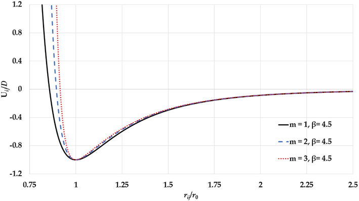
The generalized L-J potential curves for different values of the
parameter and a fixed value of the
parameter presented as a function of reduced relative distance between two atoms.
The cohesive energy per atom of the nanoparticles can found using the following formula (Kittel, 2005):
The equilibrium value of the reduced nearest distance between two atoms
is
that can be obtained by minimizing Eq. (5) is as follows:
For
, the equilibrium reduced nearest distance between two atoms
is:
However, the equilibrium relative distance for is obtained numerically.
The cohesive energy per atom in the equilibrium configuration is:
The relative cohesive energy of a nanoparticle is the ratio between the cohesive energy per atom and the cohesive energy of the corresponding bulk material
:
where
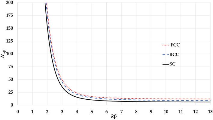
The variation of potential parameter
for different cubic structures with the
parameter.
3 Results and Discussion:
3.1 Non-integer L-J potential:
The cohesive energies of nanoparticles in an FCC structure are calculated based on the non-integer L-J potential function that is given by Eq. (2) for two different values of
parameters and compared to the cohesive energies that were calculated using the Morse Potential (Eq. (3) with
) for two different values
and
with the aim to predict the cohesive energy of a W and Mn nanoparticle respectively (Aldossary and Al Rsheed, 2020a) as seen in Fig. 3. Moreover, the calculated cohesive energies are also compared to the experimental values for the cohesive energy of Mo (0.686 for
atoms) and W nanoparticles (0.751 for
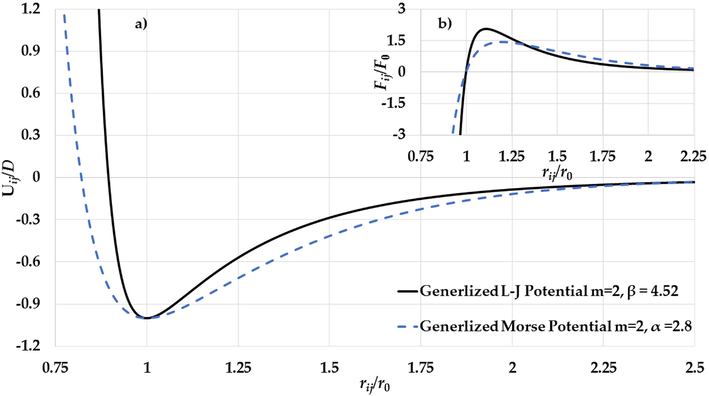
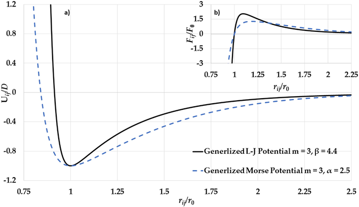
atoms) (Kim et al., 2002, Edgar, 1993). The calculated cohesive energies using the non-integer L-J potential agree with the experimental values for the cohesive energies of Mo and W nanoparticles. The nanoparticle stability exhibited using the Morse Potential is due to the softening of the repulsive wall of potential energy (Aldossary and Al Rsheed, 2020a). However, the non-integer L-J potential function can predict stable nanoparticles with stiffer repulsive walls than the Morse Potential as seen in Figs. 4a and Fig. 5a. In general, the stability of the nanoparticle is a result of the equilibrium between the repulsive force (Pauli repulsion force) and the attractive force (such as attractive dipole force) that are exerting on each atom in the nanoparticle. Both forces depend on the gradient of the potential function (
). As seen in Figs. 4b and Fig. 5b, the gradient of the attractive interaction in the L-J potential is larger than in the Morse potential when the distance between two atoms is
. As result, the gradient of the long-range attractive (the attractive force) in the L-J potential when the relative distance between two atoms in equilibrium is enough strong to cancel the effect of the gradient of the repulsive wall in the L-J potential (the repulsive force). Consequently, the stability of nanoparticle is due to the large gradient of the long-range in the potential function when the relative distance between two atoms near the equilibrium.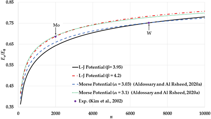
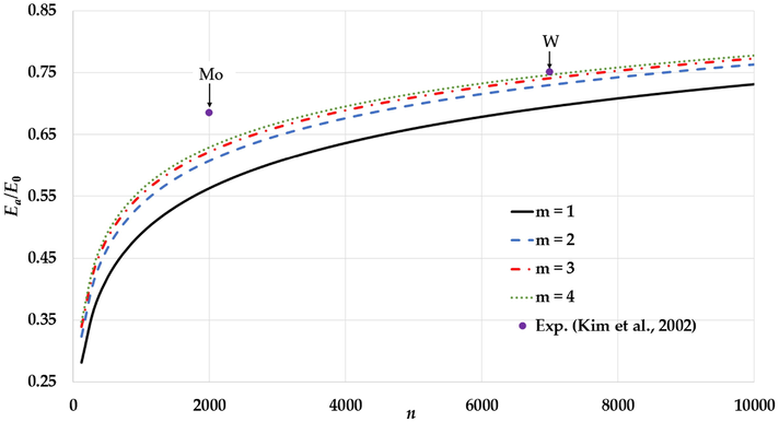
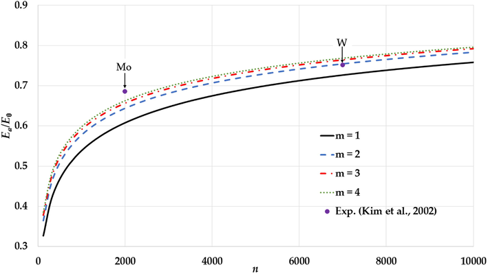
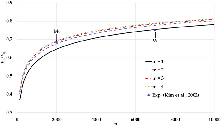
The variation of the relative cohesive energy of nanoparticles in an FCC structure as function of the number of atoms using L-J potential for different values of
and compared to the calculated relative cohesive energy using Morse potential (Aldossary and Al Rsheed, 2020a) and the experimental values of Mo and W nanoparticles (Kim et al., 2002).
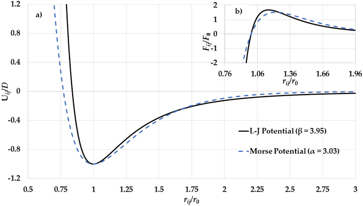
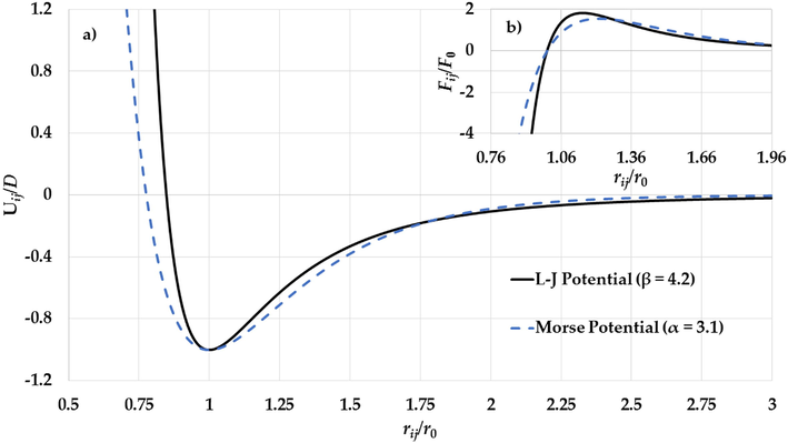
a) The potential curves of the L-J potential function (
) and the Morse potential function (
) and b) The gradient of the L-J potential function (
) and the gradient of the Morse potential function (
) (where
) as functions of reduced relative distance between two atoms.
a) The potential curves of the L-J potential function (
) and the Morse potential function (
) and b) The gradient of the L-J potential function (
) and the gradient of the Morse potential function (
) (where
) as functions of reduced relative distance between two atoms.
3.2 Generalized Non-integer L-J potential:
The generalized Non-integer L-J potential is used to calculate the cohesive energy for different values of
and fixed value of
and for different cubic structures of nanoparticles: SC as in Fig. 6 (
), Fig. 7 (
), and Fig. 8 (
); FCC as in Fig. 9 (
), Fig. 10 (
), and Fig. 11 (
); BCC as in Fig. 12 (
), Fig. 13 (
), and Fig. 14 (
). Moreover, the calculations of cohesive energies are compared to the experimental values of cohesive energy of Mo and W nanoparticles (Kim et al., 2002; Edgar, 1993). The calculations show that the value of
parameter, the value of
parameter, and the structure of nanoparticle effect on the values of cohesive energy of nanoparticle. It is found that nanoparticles with a given number of atoms (for example
atoms) can be become stable with a low value of cohesive energy if the values of
and
parameters in the generalized L-J potential function are decreased as seen in Table 1.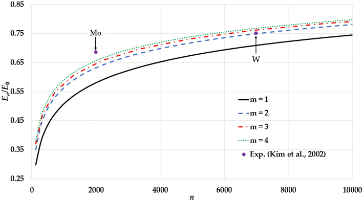
The variation of the relative cohesive energy of nanoparticles in an SC structure for different values of the
parameter and a fixed value of
parameter (
) with a comparison to the experimental values of the relative cohesive energy of Mo and W nanoparticles (Kim et al., 2002).
The variation of the relative cohesive energy of nanoparticles in an SC structure for different values of the
parameter and a fixed value of the
parameter (
) with comparisons to the experimental values of the relative cohesive energy of Mo and W nanoparticles (Kim et al., 2002).
The variation of the relative cohesive energy of nanoparticles in an SC structure for different values of the
parameter and a fixed value of the
parameter (
) with comparisons to experimental values of the relative cohesive energy of Mo and W nanoparticles (Kim et al., 2002).
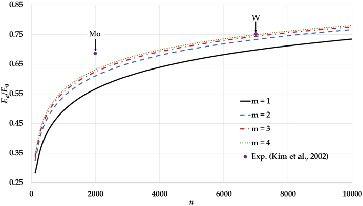
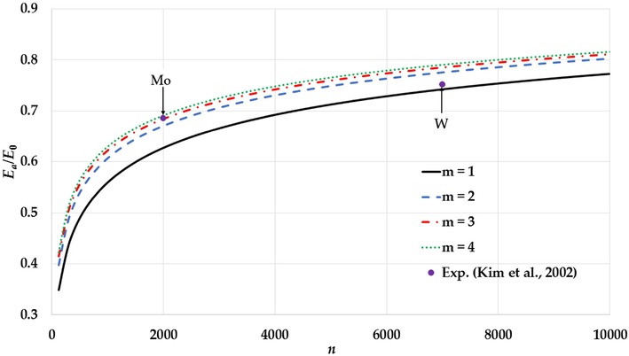
The variation of the relative cohesive energy of nanoparticles in an FCC structure for different value of the
parameter and a fixed value of the
parameter (
) with comparisons to the experimental values of the relative cohesive energy of Mo and W nanoparticles (Kim et al., 2002).
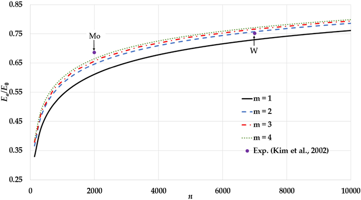
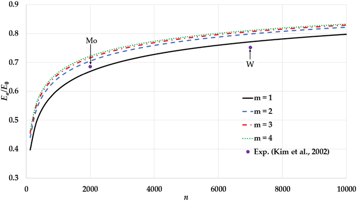
The variation of the relative cohesive energy of nanoparticles in an FCC structure for different values of the
parameter and a fixed value of the
parameter (
) with comparisons to the experimental values of the relative cohesive energy of Mo and W nanoparticles (Kim et al., 2002).
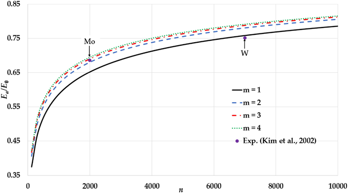
The variation of the relative cohesive energy of nanoparticles in an FCC structure for different values of the
parameter and a fixed value of the
parameter (
) with comparison to the experimental values of the relative cohesive energy of Mo and W nanoparticles (Kim et al., 2002).
The variation of relative cohesive energy of nanoparticles in an BCC structure for different value of
parameter and fixed value of
parameter (
) and compared to the experimental values of relative cohesive energy of Mo and W nanoparticles (Kim et al., 2002).
The variation of the relative cohesive energy of nanoparticles in an BCC structure for different values of the
parameter and a fixed value of the
parameter (
) in comparison to the experimental values of the relative cohesive energy of Mo and W nanoparticles (Kim et al., 2002).
The variation of the relative cohesive energy of nanoparticles in an BCC structure for different value of the
parameter and a fixed value of the
parameter (
) with comparisons to the experimental values of the relative cohesive energy of Mo and W nanoparticles (Kim et al., 2002).
Moreover, the experimental values of the cohesive energy such as for Mo nanoparticles (
for
atoms (Kim et al., 2002; Edgar, 1993)) can be successfully predicted using lager values for the
parameter if the value of the
parameter is decreased in the generalized L-J potential function as seen in Fig. 15. The values
and
parameters that can predict the experimental value of cohesive energy of Mo nanoparticle are summarized in Table 2. The values
and
parameters in the Table 2 are used to plot the potential curves as seen in Fig. 16a. The potential curves confirm that the stability of the nanoparticle with large repulsive force (large value of
parameter) is due to the large gradient in the long-range in the potential function when the relative distance between two atoms near the equilibrium as seen in Fig. 16b.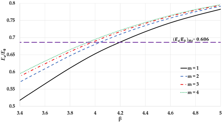
The variation of the cohesive energy using the
parameter for a nanoparticle in an FCC structure containing 2000 atoms for different values of the
parameter and a comparison with the experimental values of the cohesive energy of Mo nanoparticles (Kim et al., 2002).
1
4.2
2
4.04
3
3.98
4
3.94
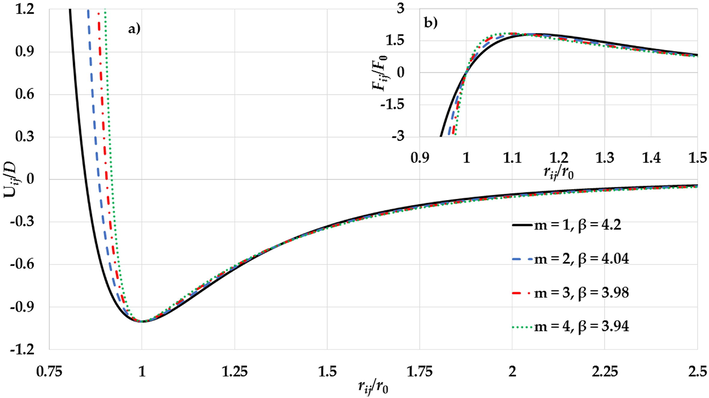
a) The potential curves of the L-J potential function and b) the gradient of the L-J potential function for different values of
and
parameters (where
) a) as functions of reduced relative distance between two atoms.
Similarly, the experimental value of cohesive energy of Mo nanoparticle was predicted by using generalized Morse potential function with large value of parameter if the value of is lowered (Aldossary and Al Rsheed, 2020b). However, the stability of the nanoparticles that was explained by using the generalized Morse potential function is due to the increased range of the attractive interaction part in the potential function.
The potential function that is given by Eq. (4) can be written in expanded form as follows:
The first parenthesis inside the curly brackets represents the repulsive interaction, whereas the second parenthesis represents the attractive interaction. The enlargement of the attractive force can be obtained by keeping the parameter large (which makes the gradient of the attractive interaction large) and the parameter small (which enlarges the range of the attractive interaction).
3.3 The melting point of Au nanoparticles:
It was reported that the cohesive energy of materials is linearly proportional to its melting point
(Dash, 1999), which is expressed as:
The melting point is a size-dependent property of nanoparticles (Buffat and Borel, 1976; Dick et al., 2002; Qi, 2005) which can be written as a function of the number of atoms
. Therefore, the ratio of the melting point of nanoparticles with
atoms to the bulk melting point equals to the relative cohesive energy (
), and using Eq. (10) to get:
The ratio
is calculated using Eq. (14) for nanoparticles in an FCC structure as a function of the number of atoms
for different values of the
and
parameters: Fig. 17 (
and
), Fig. 18 (
and
), and Fig. 19 (
and
). The results are compared to the calculations of the same ratio using the generalized Morse Potential (Aldossary and Al Rsheed, 2020b) for different values of
and
parameters: Fig. 17 (
and
), Fig. 18 (
and
), and Fig. 19 (
and
). Moreover, the calculations also are compared to two different experimental sets of melting points of Au nanoparticles (the mass density is
(Haynes, 2005) and the bulk melting point is
(Buffat and Borel, 1976)). The first of the experimental data represents the melting point of Au nanoparticles deposited on an amorphous carbon substrate (Buffat and Borel, 1976). The second set of the experimental data represents the melting point of silica-encapsulated Au nanoparticles (Dick et al., 2002). The accuracy for the first set of the experimental data for the larger Au nanoparticles is better than for the smaller Au nanoparticles because of the effect of the substrate (Lee et al., 2005). On other hand, the second set has good accuracy with small Au nanoparticles because the silica shell does not influence the melting point for the small Au nanoparticles (Dick et al., 2002).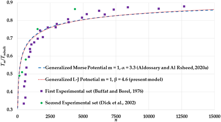
The variation of the ratio
of nanoparticles in an FCC structure using the Morse potential function (
) and the L-J potential function (
) with the same value of
with comparison to two experimental sets of melting points of Au nanoparticles (Buffat and Borel, 1976; Dick et al., 2002).
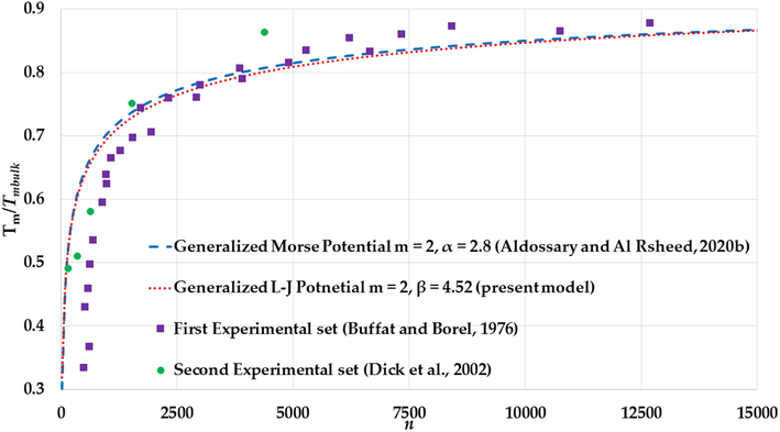
The variation of ratio
of nanoparticles in an FCC structure using Morse potential function (
) and L-J potential function (
) with the same value of
with comparison to two experimental sets of melting points of Au nanoparticles (Buffat and Borel, 1976; Dick et al., 2002).
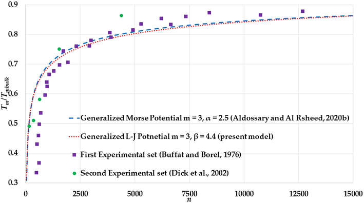
The variation of ratio
of nanoparticles in an FCC structure using the Morse potential function (
) and the L-J potential function (
) with the same value of
and comparison to two experimental sets of melting points of Au nanoparticles (Buffat and Borel, 1976; Dick et al., 2002).
The melting points for both sets are given as function nanoparticles diameters , however, the number of atoms of nanoparticle in an FCC structure with given diameters can be found using the following relation: (Safaei, 2010a; Safaei et al., 2007), where is the atomic diameter. The calculation of the melting points (with different values of and parameters) in Figs. 17–19 show an agreement with the experimental values of the melting points of the large Au nanoparticles (Au nanoparticles that have atoms) from the first experimental set and disagreement with the small Au nanoparticles due to the substrate effect. On the contrary, the calculations of melting points show an agreement with the experimental values of melting points of the small Au nanoparticles (Au nanoparticles that have atoms) from the second experimental set.
The values of
,
(for L-J potential function), and
(for Morse potential function) parameters that predict the experimental values of melting points of Au nanoparticles in Figs. 17–19 are used to plot the potential curves of the L-J potential function and the Morse potential function as seen in Figs. 20–22a. As seen in Figs. 20a–22a, the range of the attractive interaction part in the L-J potential function is similar as in the Morse potential function which plays an important role in the stability of the nanoparticles (Aldossary and Al Rsheed, 2020b). On other hand, the repulsive walls in the L-J potential function are stiffer than in the Morse potential function. Moreover, the gradient of the attractive interaction in the L-J potential is larger than that in the Morse potential when
as seen in Figs. 20b–22b. When the value of the
parameter in the L-J potential function increases then the repulsive wall becomes stiffer and the gradient of the attractive interaction part in the potential becomes high when
. As result, the high gradient of the attractive interaction in the L-J potential function when
. plays an important role in the stability of the nanoparticles.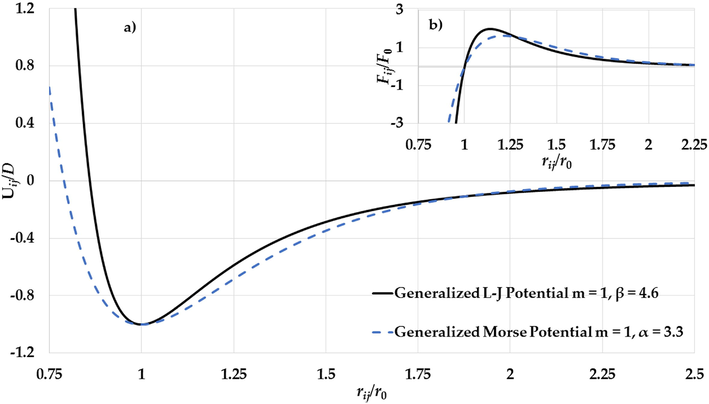
a) The potential curves of the generalized L-J potential function (
,
) and the generalized Morse potential function (
) and b) The gradient of the generalized L-J potential function (
) and the gradient of the generalized Morse potential function (
) (where
) as a functions of reduced relative distance between two atoms.
a) The potential curves of the generalized L-J potential function (
,
) and the generalized Morse potential function (
) and b) The gradient of the generalized L-J potential function (
) and the gradient of the generalized Morse potential function (
) (where
) as functions of the reduced relative distance between two atoms.
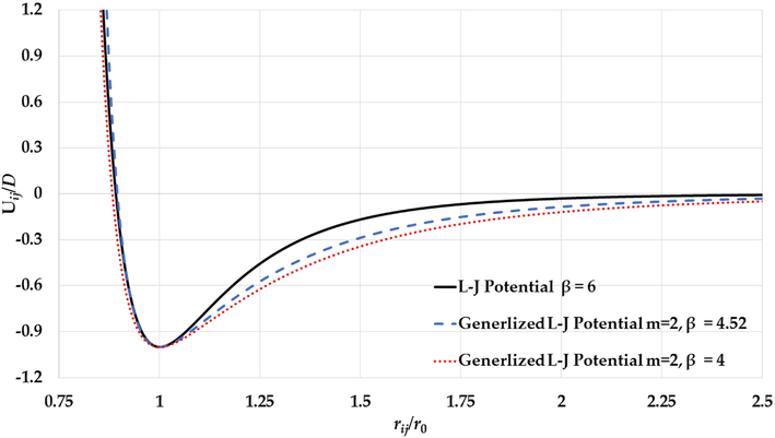
The potential curves of the L-J potential function (
), the generalized L-J potential functions (
,
) and (
) as functions of the reduced relative distance between two atoms.
4 Conclusions
The non-integer Lennard-Jones (L-J) potential function and its generalized form can be used to predict the cohesive energies and the melting points of nanoparticles. The values of the calculated cohesive energies and the melting points of nanoparticles depend on the values of the L-J potential parameters and and the structure of the nanoparticles due to the existence of the lattice structure . It is found that the nanoparticles can be stable with low cohesive energy if the parameters and are decreased.
The repulsive wall in the generalized non-integer L-J potential function is stiffer than in the generalized Morse potential function. Therefore, the stability of the nanoparticles based on the generalized non-integer L-J potential function is because of two conditions that cancel the Pauli repulsive force: The first condition is the enlargement in the attractive interaction range of the potential function (which is also satisfied in the generalized Morse potential function). The second condition is the high gradient of the attractive interaction part in the L-J potential function when .
The generalized non-integer L-J potential function with can predict the experimental values of the cohesive energies of Mo and W nanoparticles when and respectively, and the melting points of Au nanoparticles when . The repulsive walls of the generalized non-integer L-J potential function with and between and is around the repulsive wall of the L-J potential function as seen in Fig. 23. The repulsive wall of the generalized non-integer L-J potential function with represents the Pauli repulsive force in the L-J potential function (Lennard-Jones, 1924).
The generalized non-integer L-J potential function with is a useful form of the potential function to explain the bonds between the atoms in the nanoparticles. This work can push the scientific research forward by producing more experimental data that can be used to find the parameter of the generalized non-integer L-J potential function using fitting procedure as it was done for diatomic molecules (Coxon and Hajigeorgiou, 2010).
Acknowledgment
Researchers supporting project number (RSP- 2020/61), King Saud University, Riyadh, Saudi Arabia.
Declaration of Competing Interest
The authors declare that they have no known competing financial interests or personal relationships that could have appeared to influence the work reported in this paper.
References
- Abdullah, B.J., Omar, M.S., Jiang, Q., 2018. Size Effects on Cohesive Energy, Debye Temperature and Lattice Heat Capacity from First-Principles Calculations of Sn Nanoparticles. Proc. Natl. Acad. Sci., India, Sect. A Phys. Sci. 88, 629–632.
- The effect of the parameter α of Morse potential on cohesive energy. J. King Saud Univ.–Sci.. 2020;32:1147-1151.
- [Google Scholar]
- Aldossary, O.M., Al Rsheed, A., 2020b, A new generalized morse potential function for calculating cohesive energy of nanoparticles energies 13, 3323(1–16).
- Barakat, T., Al-Dossary, O.M., Alharbi, A.A., 2007. The effect of Mie-type potential range on the cohesive energy of metallic nanoparticles. Int. J. Nanosci. 6, 461–466.
- Size effect on the melting temperature of gold particles. Phys. Rev. A. 1976;13(6):2287-2298.
- [Google Scholar]
- Coxon, J.A., Hajigeorgiou, P.G., 2010. The ground X1 electronic state of the cesium dimer: Application of a direct potential fitting procedure. J. Chem. Phys. 132, 094105 (1–17).
- Dattani, N.S., 2015a. Beryllium monohydride (BeH): Where we are now, after 86 years of spectroscopy. J. Mol. Spect. 311, 76–83.
- Dattani, N.S., 2015b. Analytic potentials and vibrational energies for Li2 states dissociating to Li(2S) + Li(3P). Part 1: The 2S+1Πu/g states. arXiv:1509.07041.
- Dattani, N.S., 2018. http://hdl.handle.net/2142/100778.
- A DPF data analysis yields accurate analytic potentials for Li2(a3Σu+) and Li2(13Σg+) that incorporate 3-state mixing near the 13Σg+ state asymptote. J. Mol. Spect.. 2011;268:199-210.
- [Google Scholar]
- Dattani, N.S., Le Roy, R.J., 2015. State of the art for ab initio vs empirical potentials for predicting 6e− excited state molecular energies: Application to Li2 (b, 13Πu). arXiv:1508.07184.
- Dattani, N.S., Puchalski, M., 2014. On the empirical dipole polarizability of He from spectroscopy of HeH+. arXiv:1410.4895v1.
- Dattani, N.S., Zack, L.N., Sun, M., Johnson, E.R., Le Roy, R.J., Ziurys, L.M., 2014. Global empirical potentials from purely rotational measurements. arXiv:1408.2276
- Davari, M., Jabbareh, M.A., 2020. Modeling the interfacial energy of embedded metallic nanoparticles. J. Phys. Chem. Solids 138, 109261(1–7).
- Size-dependent melting of silica-encapsulated gold nanoparticles. J. Am. Chem. Soc.. 2002;124:2312-2317.
- [Google Scholar]
- Modeling the size dependency of the stability of metal nanoparticles. J. Phys. Chem. C. 2019;123:25464-25469.
- [Google Scholar]
- Periodic Table of the Elements. Oregon: Gaston; 1993.
- Application of the Morse potential function to cubic metals. Phys. Rev.. 1959;114:687-690.
- [Google Scholar]
- Haynes, W.M., 2005. Thermal and physical properties of pure metals. In: Lide, D.R. (Ed.), CRC Handbook of Chemistry and Physics, Internet Version;; CRC Press: Boca Raton, FL, USA.
- Size-dependent melting properties of tin nanoparticles. Chem. Phys. Lett.. 2006;429:492-496.
- [Google Scholar]
- The cluster size dependence of thermal stabilities of both molybdenum and tungsten nanoclusters. Chem. Phys. Lett.. 2002;354:165-172.
- [Google Scholar]
- Introduction to Solid State Physics (8th ed.). New York, NY, USA: Wiley; 2005.
- Le Roy, R.J., Dattani, N.S., Coxon, J.A., Ross, A.J., Crozet, P., Linton, C., 2009. Accurate analytic potentials for Li2(X1) and Li2(A1) from 2 to 90 Å, and the radiative lifetime of Li(2p). J. Chem. Phys. 131, 204309(1–17)
- An accurate analytic potential function for ground-state N2 from a direct-potential-fit analysis of spectroscopic data. J. Chem. Phys.. 2006;125:164310.
- [Google Scholar]
- Thermodynamic study on the melting of nanometer-sized gold particles on graphite substrate. J. Mater. Sci.. 2005;40:2167-2171.
- [Google Scholar]
- Analytic Morse/long-range potential energy surfaces and predicted infrared spectra for CO2–H2. J. Chem. Phys.. 2010;132:214309.
- [Google Scholar]
- Little, S.A., Begou, T., Collins, R.W., Marsillac, S., 2012. Optical detection of melting point depression for silver nanoparticles via in situ real time spectroscopic ellipsometry. Appl. Phys. Lett. 100, 051107(1–4).
- Predicting the size- and shape-dependent cohesive energy and order-disorder transition temperature of Co-Pt nanoparticles by embedded-atom-method potential. J. Nanosci. Nanotech.. 2013;13:1261-1264.
- [Google Scholar]
- Diatomic molecules according to the wave mechanics. II. Vibrational levels. Phys. Rev.. 1929;34:57-64.
- [Google Scholar]
- Structural stability of ruthenium nanoparticles: a density functional theory study. J. Phys. Chem. C. 2017;121:27445-27452.
- [Google Scholar]
- Improved cohesive energy of metallic nanoparicles by using L-J potential with structural effect, Iran. J. Sci. Technol. Trans. Sci.. 2019;43:2705-2711.
- [Google Scholar]
- A comprehensive understanding of melting temperature of nanowire. Nanoscale. 2012;4:2748-2753.
- [Google Scholar]
- Pawlow, P., 1909. Über die Abhängigkeit des Schmelzpunktes von der Oberflächenenergie Eines Festen. Körpers. Z. Phys. Chem. 65, 1–35.
- Size effect on melting temperature of nanosolids. Phys. B: Condens. Matter. 2005;368:46-50.
- [Google Scholar]
- Size and shape dependent melting temperature of metallic nanoparticles. Mater. Chem. Phys.. 2004;88:280-284.
- [Google Scholar]
- Calculation of the cohesive energy of metallic nanoparticles by the Lennard–Jones potential. Mater. Lett.. 2004;58:1745-1749.
- [Google Scholar]
- Surface-area-difference model for thermodynamic properties of metallic nanocrystals. J. Phys. D: Appl. Phys.. 2005;38:1429-1436.
- [Google Scholar]
- Size-dependent cohesive energy, melting temperature, and Debye temperature of spherical metallic nanoparticles. Phys. Metals Metallogr.. 2017;118:528-534.
- [Google Scholar]
- The effect of the averaged structural and energetic features on the cohesive energy of nanocrystals. J. Nanopart. Res.. 2010;12:759-776.
- [Google Scholar]
- Shape, Structural, and energetic effects on the cohesive energy and melting point of nanocrystals. J. Phys. Chem. C. 2010;114:13482-13496.
- [Google Scholar]
- Safaei, A., Shandiz, M.A., Sanjabi, S., Barber, Z.H., 2007. Modelling the size effect on the melting temperature of nanoparticles, nanowires and nanofilms. J. Phys.: Condens. Matter 19, 216216 (9pp).
- Thermodynamics of melting and freezing in small particles. Surf. Sci.. 1995;341:40-50.
- [Google Scholar]
- A simplified model to calculate the surface-to-volume atomic ratio dependent cohesive energy of nanocrystals. J. Phys.: Condens. Matter. 2004;16:L401-L405.
- [Google Scholar]
- Size-dependent melting point depression of nanostructures: Nanocalorimetric measurements. Phys. Rev. B. 2000;62:10548-10557.
- [Google Scholar]
- Yeshchenko, O.A., Dmitruk, I.M., Alexeenko, A.A., Dmytruk, A.M., 2007. Size-dependent melting of spherical copper nanoparticles embedded in a silica matrix. Phys. Rev. B 75, 085434(1–6).


