Gaussian models for anthropogenic CO₂ emissions consistent with prescribed climate targets

2.1 Quadratic interpolation

Classically, a quadratic interpolation consists of determining a quadratic function using the values that it takes on at exactly three particular values of its variable. The following result provides an original quadratic interpolation using also three given data on the parabola representing the function: its axis of reflection, one of its points (other than the vertex), and the slope of the tangent line at that point. This technique will be used to add a smooth transition to a Gaussian decline of CO₂ emissions.

If a parabola is symmetric about the line: $x=u$, passes through a point $(x_0,y_0)$, with $x_0\ne u$, and is tangent at this point to the line of slope m, then an equation of this parabola is:

2.2 Gaussian models and their integration

Gaussian models were introduced in probability theory by C. F. Gauss; considered as one of the greatest mathematicians of all time, for real-valued random variables “normally” distributed with mean $\mu$ and variance ${\sigma }^2$. These models are of the form:$$f_{\mu ,\sigma }(t)={\mathit{Ke}}^{-{(t-\mu )}^2/2{\sigma }^2}(K>0)\text{.}$$

Compared with exponential models, which are of the form ${\mathit{Ke}}^{-\alpha (t-\mu )}(\alpha >0)$, they decrease much more rapidly over the interval $(\mu +\alpha \sigma ,\infty )$. Indeed, whereas the relative rate of decline remains constant ($\alpha$) for the latter, that of the former ($\frac{t-\mu }{\sigma }$) increases indefinitely from its minimum level $\alpha$. Such a difference will help to design more suitable models by either advancing the ‘zero’ timing of CO₂ emissions or lowering and advancing their peak.

The special case where $K=1/\sqrt{2\pi },\mu =0$, and $\sigma =1$ gives the standard Gaussian probability density function f used to define the standard Gaussian cumulative distribution function $\mathrm{\Phi }$ by:$$\mathrm{\Phi }(x)=p(X⩽x)={\int }_{-\infty }^{x}f(t)\mathit{dt},$$which takes on the particular value $1/2$ at 0 and has 0 and 1 as lower and upper limits. More generally, for a given number between 0 and 1, thus, considered as an intermediate value of the continuous function $\mathrm{\Phi }$, an estimation of the corresponding x value is provided in the standard normal distribution table, also called Z table. Conversely, the same table can be used to estimate $\mathrm{\Phi }$ at a given value of x. On the other hand, the substitution $z=\frac{t-\mu }{\sigma }$ gives a typical integral of a general Gaussian model in terms of specific values of the function $\mathrm{\Phi }$ as follows:

Such formulation will be used to design and refine Gaussian pathways for CO₂ emissions consistent with a prescribed climate target.

2.3 No-mitigation scenario and remaining CO₂ Budget

The consistency of future CO₂ emissions with a prescribed climate target (defined as a target limit to the rise in temperature) and their rapid reduction, as urged by the UN, are crucial in the elaboration of suitable pathways for the emissions. Prior to their modelling, however, three predictions in the beginning of the mitigation (at time $t=t_0$) are needed; their level $G_0$, their rate of growth ${\alpha }_0$, and the remaining CO₂ budget R associated with the climate target. By definition, the CO₂ budget is the total amount of cumulative anthropogenic CO₂ emitted in the atmosphere since the industrial revolution up to the time h when the UN climate target will be hit (under the assumption of no climate mitigation). An explicit formula of this date (h) in terms of the climate target is available in (Jaoua, 2020). To estimate the remaining budget at any time, future emissions need to be modelled explicitly with time under the assumption of no climate policy, which can be done by a linear regression of the annual gas emissions since 2000 using Carbon Dioxide Information Analysis Center (CDIAC) database (Marland et al., 2016). This leads to the following no-climate-policy model $G_0$ (in GtCO₂), applicable from the year 2000 ($t=0)$:

Such linear regression was found to be statistically highly significant ($p<{10}^{-11})$ and extremely strong ($r^2\approx 0.98)$. As a consequence of Eq. (3), the remaining CO₂ budget $R(t)$, from time $t(0⩽t<h)$, consistent with the given climate target, is estimated as follows:

In particular, the remaining CO₂ budgets from 2020, to meet the targets 1.5 °C and 1.8 °C, will be estimated at 1155 and 2929 (GtCO₂ respectively, and these represent about 63$\%$ and 81$\%$ of the corresponding remaining budgets from 2000.

3.1 Gaussian model without transition

Graphically, the right-half of a suitable bell can be suggested as a possible smooth pathway for CO₂ emissions reduction regardless of the ‘zero’ timing, which will limit the rise in annual temperature to below the prescribed climate target. This gives a Gaussian model without transition, consistent with that target, defined by:

Despite the consistency of the model $G_1$ with the climate target, the emissions could not be brought close to zero as early as needed; not even before the 23rd century for the 1.8 °C target. But this delay is, in fact, much shorter than the one expected from an exponential model (Fig. 1). Nevertheless, a smooth transitional slowdown will expedite the Gaussian reduction, and thus, shorten and even avoid such delay.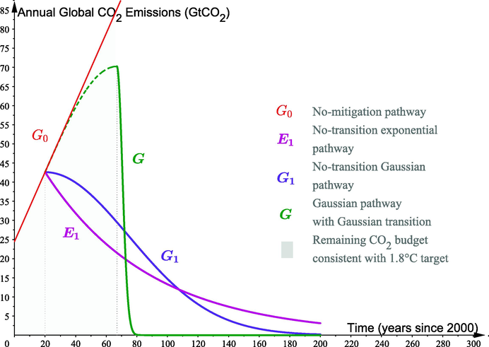

Close

Fig. 1

Gaussian and exponential models, for global CO₂ emissions, consistent with the 1.8 °C target (mitigation starting in 2020).

Export to PPT

3.2 Gaussian model with Gaussian transition

A portion of the left half of a suitable bell will be of great use to ensure a smooth transition to a Gaussian decline. More precisely, for a given climate target above a specific future warming level l expected to be hit due to a total amount r of unmitigated CO₂ emissions from time $t_0$, one can suggest the following as a unique mitigated-emissions model G, with Gaussian slowdown and decline, consistent with such a climate target:

To fit the predicted level of emissions at $t_0$, the inflection time $\mu -{\sigma }_1$ must be set at $t_0$, and this gives the relation $\mu$ vs. ${\sigma }_1$. The coefficient A can then be determined by taking this into account along with the prediction $G_0$ at $t_0$. On the other hand, the transition to the Gaussian trend must occur smoothly at $t_0$, which means that the rates of growth of the emissions must be the same at $t_0^{-}$ at $t_0^{+}$. In other words, $G_0/{\sigma }_1={\alpha }_0$, and this gives the parameter ${\sigma }_1$.

To determine the other parameter ${\sigma }_2$, one can split the remaining CO₂ budget into two parts: one $(\mathit{pR})$ for the decline and the other $\left((1-p)R\right)$ for the transition ($0<p<1$). Considering the restriction of the model G to the time interval $(\mu ,\infty )$, one gets an analogous version of the model $G_1$ with the parameters $\mathit{pR},A,\mu$ and ${\sigma }_2$ instead of $R,G_0,t_0$ and $\sigma$ respectively. Therefore, ${\sigma }_2$ can be derived by analogy from Eq. (5): ${\sigma }_2=\sqrt{2/\pi }\mathit{pR}/A$. Now, plug in $G_0\sqrt{e}$ for A to get:

The exact expression of p will be determined by solving the CO₂ budget equation that corresponds to the transition period:$${\int }_{t_0}^{\mu }G(t)\mathit{dt}=(1-p)R\text{.}$$

According to Eq. (2) for $K=A,\sigma ={\sigma }_1,a=t_0$, and $b=\mu$, this is equivalent to:$$A{\sigma }_1\sqrt{2\pi }\left(\mathrm{\Phi }(0)-\mathrm{\Phi }\left(\frac{t_0-\mu }{{\sigma }_1}\right)\right)=(1-p)R\text{.}$$

By taking into account the expressions found for A and ${\sigma }_1$ and the relations: $\mu =t_0+{\sigma }_1,\mathrm{\Phi }(0)=1/2$, and $\mathrm{\Phi }(-1)=1-\mathrm{\Phi }(1)$, one gets: $(1-p)R=r$, where $r=\sqrt{2\pi e}\left(\mathrm{\Phi }(1)-1/2\right)G_0^2/{\alpha }_0$. This gives $p=1-(r/R)$, which is in the interval $(0,1)$, due to the assumption made on the climate target. The announced formula for ${\sigma }_2$ follows immediately by plugging in $1-(r/R)$ for p in Eq. (7). The model G is unique since p is uniquely determined.

The pathway G, as given in Eq. (6), reflects a better mitigation than $G_1$ does, due to a smooth transition prior to a much faster reduction to almost zero. Indeed, according to G for the 1.8 °C target, the emissions will be brought to nearly zero in the early 2080s if their mitigation starts in 2020. This cannot happen through the pathway $G_1$ before the 23rd century (Fig. 1) and not even for the lower target 1.5 °C before the 22rd century. Unfortunately, G only fits the climate targets set up above a certain warming level l, which is estimated at about 1.76 °C for a mitigation starting in 2020. Besides, the emissions are expected to peak at a very high level, e.g., around 70.3 GtCO₂ for the 1.8 °C target (Fig. 1), thus, about 2.9 times the 2000 record. However, a suitable adjustment of the model G will not only help to include all climate targets, but will also provide an uncountable variety of models that project more appropriate emission peaking and ‘zero’-emission timing.

3.3 Gaussian models with quadratic transition

Following the same idea behind the previous modelling, a parameter $\gamma (0<\gamma <1)$ is also introduced here to split the remaining budget into two parts: $(\gamma R)$ for the Gaussian decline and $\left((1-\gamma )R\right)$ for the transition, which is, unlike in the model G, quadratic rather than Gaussian. This refinement brings a certain flexibility to the modelling (due to the arbitrariness of $\gamma$), which will help to determine optimal pathways for the lowest emissions peak and earliest ‘zero’ emission. The resulting parametrised model $G_{\gamma }$ can be stated as follows:

Indeed, let $\mu =t_0+\tau$, where $\tau >0$ denotes the total duration of the transition. The coefficients A and B follow immediately from Eq. (1) applied with $(x_0,y_0,u)=(t_0,G_0,\mu )$ and $m=\frac{{\mathit{dG}}_{\gamma }}{\mathit{dt}}{|}_{t=t_0}=\frac{{\mathit{dG}}_0}{\mathit{dt}}{|}_{t=t_0}={\alpha }_0$ (for transition smoothness). One can then determine $\sigma$ using the same argument that led to the coefficient ${\sigma }_2$ in the model G. To find the transition period, one needs to write and solve, for $\tau$, the CO₂ budget equation related to the transition phase:$${\int }_{t_0}^{\mu }{G}_{\gamma }(t)\mathit{dt}=(A/3){\tau }^3+B\tau =(1-\gamma )R\text{.}$$

By taking into account the expressions of A and B then simplifying, one gets the following equation:

The discriminant $\mathrm{\Delta }$ of this quadratic equation is given by: $\mathrm{\Delta }=G_0^2+4{\alpha }_0(1-\gamma )R/3$ and satisfies the condition: $\mathrm{\Delta }>G_0^2>0$, which gives its unique positive solution: $\tau =(-G_0+\sqrt{\mathrm{\Delta }})/(2{\alpha }_0/3)=3(-G_0+\sqrt{\mathrm{\Delta }})/(2{\alpha }_0)$, as announced in Eq. (8).

In the limit case where $\gamma =0$ (no-mitigation scenario), the model $G_{\gamma }$ degenerates into the linear pathway $G_0$ represented in Fig. 1. However, in the other limit case where $\gamma =1$ (no-transition scenario), the model is reduced to the 1-phase Gaussian pathway $G_1$ given in Eq. (5) and graphed in Fig. 1.

Notes

1. In the setting of moderate climate targets such as 1.8 °C, the flexible pathway $G_{\gamma }$ will permit to limit the emissions at a lower level than expected from the model G. For instance, as shown in Table 1, the emissions are projected to peak below 2.5 (2.65) times the record of the year 2000 for $\gamma >.2315(.0386)$, compared to 2.9 times with the model G (see Fig. 1). In addition, the ‘zero’-emission timing (i.e., when the emissions will be brought to below 0.01 GtCO₂) can be projected earlier than expected from the pathway G, e.g., before the year 2080 for the 1.8 °C target. According to Table 1, this is ensured by any model $G_{\gamma }$ for $\gamma <.0839$. As for the class of $G_{\gamma }$s, the smaller the $\gamma$, the higher and later the peak, and the earlier the zero emission.

2. For the 1.5 °C target, the models $G_{\gamma }$, with $\gamma \approx 1$, project low emissions (less than 1 GtCO₂) by 2080, similarly to half of the RCP2.6 models ([, Rogelj et al.2018), with the advantage of reducing the emissions (almost immediately) smoothly and nearly ending them by 2090. On the other hand, Fig. 2 shows that the pathway $G_{.1277}$ will bring the emissions to ‘zero’ in 2050, that is, earlier than expected from the (IPCC) no/limited/higher overshoot models without CO₂ removal as required in the latter to meet the climate target (IPCC, 2018). Moreover, $G_{.0566}$ will bring the emissions from a slightly higher peak ($\approx$ 52.65 GtCO₂) to ‘zero’ ($\sim$2046) in only 4 years instead of about 10 years, which explains its lower feasibility (see Fig. 2). When considering a lower target such as 1.4 °C, as shown in Fig. 2, $G_{.1366}$ and $G_{.0506}$ will permit to advance the zero timing to the years 2040 and 2037 respectively, even though the former seems more realistic than the latter due to its longer period between the peak and ‘zero’ timings (7 years vs. 2 years). More generally, $G_{\gamma }$s reflect a better mitigation, not only for projecting a lower (and/or earlier) peaking (compared to G) and/or an earlier ‘zero’-emission (compared to IPCC models), but also for slowing the emissions smoothly before their reduction, which will help to ease the decarbonisation of the economy.

3. When it comes to the ideal $G_{\gamma }$s for a given climate target, their selection depends on specific criteria such as ‘zeroing’ the emissions before a prescribed year and/or limiting them below a certain level (compared to the record in the year 2000). The selection outcomes based on these criteria are presented in Table 1. According to this table, the $G_{\gamma }$s, for $.0386<\gamma <.0839$, are found to be an ideal match for the 1.8 °C target, as they will make the emissions peak below 2.65 times the 2000 level and bring them to nearly zero before the year 2080. For a climate target as close as 1.5 °C (resp. 1.4 °C), compared to a predicted warming of about 1.2 °C for 2020 (see Jaoua, 2020), another range of $G_{\gamma }$s $\left(.0593<\gamma <.1277(\mathit{resp}..0965<\gamma <.1366)\right)$ is found to be the pattern that will help to limit the emissions below 2.15 times (resp. twice) the 2000 record and reduce them to almost zero before the year 2050 (resp. 2040).

4. The feasibility of $G_{\gamma }$ can be improved by keeping the highest annual reduction below a sensible level, such as twice the average annual reduction already achieved by each of the EU and USA (since 2005), i.e., $2\times 2.8=5.6$ GtCO₂ (see EESI, 2018). Given the Gaussian trend, the annual reduction will reach its maximum at the inflection time $t=\mu +\sigma$. Therefore, one may consider $G_{\gamma }$ realistic whenever it satisfies the following condition:$$G_{\gamma }(\mu +\sigma -1)-G_{\gamma }(\mu +\sigma )<6$$which sets $\gamma$ in the interval $(.2761,1)$ for the 1.5 °C target. Among these models, $G_{.2762}$ would be the best fit for the earliest feasible zero-emission which will occur in 2058, with an average annual reduction of less than 2.5 GtCO₂. More or less feasible pathways are presented in Table 2 in which three zero-emission timings are considered: 2050, 2055, and 2060.

5. Limitations of the $G_{\gamma }$s: although optimal peaks and zero timings for the emissions can be determined thanks to the flexibility of $G_{\gamma }$, these predictions could be improved with a lower estimation of the remaining budget of CO₂ emissions. In fact, the estimation used in this study is based on an overestimation of the date h at which the prescribed climate target would be hit in the no-mitigation scenario, and this is due to the non consideration of further greenhouse gases in the global warming model used to predict this date. On the other hand, the $G_{\gamma }$s do not cover any failure of the associated climate action, due for example to the countries which are not part of or will cease their participation in the Paris agreement on climate change. This could ultimately lead to an extended networked version of the models.

Close

Fig. 2

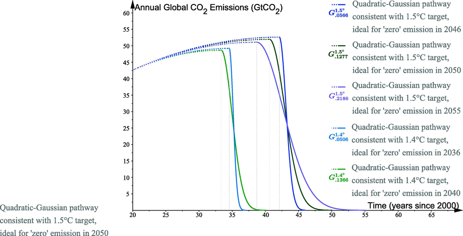
Gaussian models, with quadratic transition, for global CO₂ emissions, consistent with the climate targets 1.5 °C and 1.4 °C and specific ‘zero’-emission timings mitigation starting in 2020.

Export to PPT

References

- C2ES, 2018. Center for Climate and Energy Solutions. Main Greenhouse Gases. Technical report, C2ES. URL:https://www.c2es.org/content/main-greenhouse-gases.
- EESI, 2018. US leads in GHG. Reduction. Environmental Energy Study Institute. URL:https://www.eesi.org/articles/view/u.s-leads-in-greenhouse-gas-reduction-but-some-states-are-fallingbehind.
- An investigation of the oxidative dehydrogenation of propane kinetics over a vanadium-graphene catalyst aiming at minimizing of COx species. Chem. Eng. J.. 2014;250(15):14-24.
- [CrossRef] [Google Scholar]
- IPCC, 2014. Intergovernmental Panel on Climate Change. Climate Change 2014, The Fifth Assessment Report, AR5-SPM. Cambridge University Press, Cambridge and New York.
- IPCC, 2018. Summary for Policymakers. Global Warming of 1.5 °C. An IPCC Special Report on the impacts of global warming of 1.5 °C above pre-industrial levels and related global greenhouse gas emission pathways, in the context of strengthening the global response to the threat of climate change, sustainable development, and efforts to eradicate poverty. [Masson-Delmotte, J. et al. (editors)]. World Meteorological Organization, Geneva, 32.
- Climate Mitigation Mathematical Models Consistent with the 2015 Paris Agreement. Int. J. Global Warming. 2020;21(3):287-298.
- Jones, C.D., Arora, V., Friedlingstein, P., Bopp, L., Brovkin, V., Dunne, J., Graven, H., Hoffman, F., Ilyina, T., John, J.G., Jung, M., Kawamiya, M., Koven, C., Pongratz, J., Raddatz, T., Randerson, J.T., Zaehle, S., 2016. C4MIP – The Coupled Climate–Carbon Cycle Model Intercomparison Project: experimental protocol for CMIP6. Geoscientific Model Development, 9 (8), 2853–2880.
- Jubb, I., 2016. Representative Concentration Pathways (RCPs). Australian Climate Change. Science Program. URL:http://www.cawcr.gov.au/projects/Climatechange/wp-content/uploads/2016/11/ACCSP.
- Knutti, R., 2013. Relationship between Global Emissions and Global Temperature Rise. Climate Change 2013: The Physical Science Basis. WG1 Contribution to IPCC-AR5, Chapter 12. URL:https://unfccc.int/sites/default/files/7_knutti.reto.3sed2.pdf.
- Marland, G., Boden, T., Andres, B., 2016. Global CO2 Emissions from Fossil-Fuel Burning, Cement Manufacture, and Gas Flaring: 1751–2013. CDIAC (Carbon Dioxide Information Analysis Center). Technical report, Research Institute for Environment, Energy, and Economics, USA. URL:https://cdiac.ess-dive.lbl.gov/ftp/ndp030/global.1751_2013.ems.
- Climate change governance, cooperation and self-organization. Phys. Life Rev.. 2014;11(4):573-586.
- Scenarios towards limiting global mean temperature increase below 1.5 C. Nat. Clim. Change. 2018;8
- [Google Scholar]
- Rogelj, J., Shindell, D., Jiang, K., Fifita, S., Forster, P., Ginzburg, V., Handa, C., Kheshgi, H., Kobayashi, S., Kriegler, E., Mundaca, L., Séférian, R., Vilariño, M.V., Calvin, K., Edelenbosch, O., Emmerling, J., Fuss, S., Gasser, T., Gillet, N., He, C., Hertwich, E., Isaksson, L.H., Huppmann, D., Luderer, G., Markandya, A., McCollum, D., Millar, R., Meinshausen, M., Popp, A., Pereira, J., Purohit, P., Riahi, K., Ribes, A., Saunders, H., Schadel, C., Smith, C., Smith, P., Trutnevyte, E., Xiu, Y., Zickfeld, K., Zhou, W., 2018b. Mitigation Pathways Compatible with C in the Context of Sustainable Development. Global Warming of C. An IPCC Special Report on the impacts of global warming of C above preindustrial levels and related global greenhouse gas emission pathways, in the context of strengthening the global response to the threat of climate change, sustainable development, and efforts to eradicate poverty. [V. Masson-Delmotte, P. Zhai, H.O. Prtner, D. Roberts, J. Skea, P.R. Shukla,A. Pirani, W. Moufouma-Okia, C.Pan, R. Pidcock, S. Connors, J.B.R. Matthews, Y. Chen, X. Zhou, M.I. Gomis, E. Lonnoy, T. Maycock, M. Tignor, T. Waterfield(eds.)], in press.
- UN, 2019. 09-23 Climate Action Summit. Technical report, UN (United Nations). URL:https://www.un.org/en/climatechange/9.
- UNF, 2015. (United Nations Framework Convention on Climate Change). Paris Agreement. URL:http://unfccc.int/paris.
- Integrated workflow in 3D geological model construction for evaluation of CO2 storage capacity of a fractured basement reservoir in Cuu Long Basin, Vietnam. Int. J. Greenhouse Gas Control. 2019;90
- Robust optimization of CO2 Sequestration through a water alternating gas process under geological uncertainties in Cuu Long Basin, Vietnam. J. Natural Gas Sci. Eng.. 2020;76
- Impact of a new geological modelling method on the enhancement of the CO2 storage assessment of E sequence of Nam Vang field, offshore Vietnam. Energy Sources, Part A: Recovery, Utilization, and Environmental Effects. 2020;42(12):1499-1512.
- Vuuren, D., Edmonds, J., Kainuma, M., Riahi, K., Thomson, A., Hibbard, K., Hurtt, G., Kram, T., Krey, V., Lamarque, J.-F., Masui, T., Meinshausen, M., Nakicenovic, N., Smith, S., Rose, S., 2011. The representative concentration pathways: an overview. Climatic Change. This issue. Climatic Change, 109, 5–31.