

Translate this page into:
Frictional self-contact problem of elastic rods
-
Received: ,
Accepted: ,
This article was originally published by Elsevier and was migrated to Scientific Scholar after the change of Publisher.
Peer review under responsibility of King Saud University.
Abstract
In this article, we studied the modeling of a hyperelastic rod during large displacements in the presence of a frictional self-contact described by the Coulomb’s law. Compared to other works the self-contact subject with friction is addressed as a problem in itself. This problem generates nonlinear constraints leading to difficulties in mathematical and numerical analysis. To relax the problem of these constraints, an augmented Lagrangian method was used. As a result, we overcame the implicit nature of the Signorini-Coulomb-self-contact formulas. We presented, on the one hand, a result of the existence of the solution. On the other hand, we have proposed an approach that can be useful for a numerical implementation of this problem.
Keywords
74K10
74M15
74S05
Frictional self-contact
Gap vector
Tangential sliding velocity
Signorini-Coulomb friction

Nomenclature
- l, ε
-
Initial length and the initial radius
-
Displacements of each configuration
-
Internal force
- m
-
Internal moment
- N, T
-
normal and tangential vectors
-
Normal and tangential stresses
-
Normal and tangential penalties parameters
-
Normal and tangential penalized stresses
-
Gap vector
-
Gap function
-
Sliding velocity vector
-
Tangential friction coefficient
- p, q
-
Admissible displacement and rotation variations
1 Introduction
Several systems of mechanical structures reveal situations in which an elastic body undergoes self-contact or come in contact with other bodies. Among the recently studied systems, is the DNA supercoiling in chromatin where the change of configuration can influence their local and global structure (Gilbert and Allan, 2014). Another possible example could be the increased use of the stent in the biomedical field. For example, the use of stent-grafts for endovascular repair can lead to serious complications (Demanget et al., 2012; Demanget et al., 2013), despite the large experimental and computational studies. Another example of studying the physical structure of the collision and contact phenomena of different layers of clothing in a virtual garment of the physically based animation. This type of modelization is important to enrich realism provided by physics based simulation in animation (Jiang et al., 2017). Moreover, the nature of the contact plays a determining role in their behavior. The general theory could be attributed to (Duvaut and Lions, 1972) who gave the variational formulations of contact problems and proved the existence and uniqueness of the solution for bilateral contact problems using Tresca’s friction law. In Nečas et al. (1980), they have proved the existence of unilateral contact problem in the static state using a local Coulomb friction law. This result was extended by Jarušek (1983). For a static problem, where a law of normal conformity describes the contact, we can refer to Oden and Martins (1985) and Klarbring et al. (1989). The unilateral contact problems with non-local Coulomb friction have been studied by Duvaut (1980), Demkowicz and Oden (1982), Oden and Pires (1983), Cocu (1984) and Renard (2006). Besides, we cite the work in Béal and Touzani (2003) about the contact in large displacements. The self-contact problem had not been considered analytically as an autonomous topic in the classic scientific literature, but it is considered as a special case, which must, therefore, be dealt with accordingly. Motivated by the self-contact due to the supercoiling phenomena of DNA, the self-contact caused by the writhing of the clamped rods has been studied by Van der Heijden et al. (2003). In Chamekh et al. (2009), a result of the existence for the frictionless self-contact problem and a numerical approach have been given.
This work presents the great difficulties we face in proving even the existence of solutions to quasi-static frictional self-contact problems of elastic rods. One of our basic goals is the aim is to understand, if possible in physical terms, the meaning of non-uniqueness and non-existence in the quasi-static case. The frictional Coulomb’s law does not admit of potential, and even for Tresca’s law does not admit of potential in the case of large displacements. For this reason, we cannot prove the uniqueness and the existence of solution by the minimization of the total energy method or even if we rely on the balance equations, because we fall into a coupling between displacement and rotation, and which leads to a strong non-linearity.
We propose to extend these results to a particular result of existence whose the frictional self-contact force is known, fixed and proposed as a penalized force to ensure the uniqueness result. That is, solving the non-linear problem in the Uzawa algorithm before updating the Lagrange multipliers. This force is proposed by regularized normal and tangential vectors, this regularization is applied to the contact pressure to extend the scope of the results as well.
2 Geometrically exact rod
2.1 Preliminaries
We consider a direct orthonormal fixed frame
of the Euclidean space
. We denote by
the Euclidean norm on
. For a vector
, we associate the antisymmetric tensor
, i.e.
for all vector
. We denote by
the axial vector associated with the antisymmetric tensor, that is to say, such that
. The projection of a vector
onto a ball centered at the origin and with a radius
is defined as:
2.2 Configurations of Cosserat rods
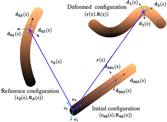
Compared to the work of Mlika et al. (2017) that has treated the frictional self-contact problem by a theory based on Nitsche’s method, we have used the geometrically exact theory (GET) which plays an important role in much recent mechanical research. This theory is based on the Cosserat’s rod (Cosserat and Cosserat, 1909), governed by the equations developed in Reissner (1981) and Simo and Vu-Quoc (1988). The GET has many benefits, has of the advantage to parametrize the 3D configuration of the rod by a 1D parametrization and to take into account the torsion, bending, elongation and shear. The GET could be based on Simo-Reissner theory that we have mentioned above, or also on the Kirchhoff-Love theory (Meier et al., 2016). The studied rod is initially defined by a right centerline (untwisted) fixed on the spatial basis , the reference configuration that is also called unstressed or stress-free configuration. However, it can be initially twisted and/or curved on the basis . Under the action of external efforts, the rod is deformed and moves from the reference configuration to the deformed configuration defined by the deformed centerline on the material basis . In this model, the sections are initially plane and remain plane with an invariant radius . The deformed configuration is then described by the position of each (with l is the initial length of the rod) which moves by a partial translational displacement , i.e. , and by translational displacement and turns with the cross-section and therefore with the local frame by the orthogonal tensor .
Consequently, the transformation
is the orthogonal tensor which determines the overall orientation of the cross-section. The diagram Fig. 1 explains the relation between these tensors.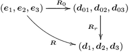
The different configurations of a Cosserat elastic rod.
Thus, the space of all possible configurations of the rod satisfying a given boundary conditions BC is
2.3 Balance equations
In what follows, we assume that the transformation is very slow so that we can neglect the forces of inertia. The time parameter must not appear even in the equilibrium equations. Nevertheless, we must use an Euler scheme to discretize the tangential velocity field in time (Mlika et al., 2017). The balance equations are the equations, which describe the variation of the internal force
and the internal moment
on the centerline of the rod. We obtain the local form of the balance equations under the action of external distributed force
and torque
for the rod writes
Concerning constitutive laws, we suppose that exists an elastic energy density
obeys the convexity and coercivity hypotheses with respect to its last two arguments (Antman, 2004) and which verify the following relationships
3 Frictional self-contact model
3.1 Self-contact problem
Generally, the self-contact do not be frictionless realized unless we neglect the tangential and rotational stress on the interface. We consider for all of the centerline of the rod the subset of of the points likely to come into contact with s. Physically, the subset defined by the points where the self-contact can take place and avoid very close points that cannot come into contact with s (Chamekh et al., 2009).
We define the normal and the tangent vectors to the curve of the centerline of the rod on the point
which describe the deformation of the rod by (see Fig. 3)
Consequently, this constraint of the non-self-penetration of material leads to the following space of kinematically and physically admissible configurations (see Fig. 2)
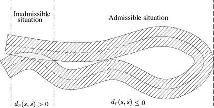
Admissible and inadmissible situations of elastic rods.
3.2 Characterization of frictional self-contact
The contact force applied between two points, which are found, respectively, on the cross-sections boundaries
and
so that we can continue the contact pressure (normal force) and the frictional efforts (tangential and rotational frictional forces) without falling in the self-penetration problem. If we neglect the rotational friction, the contact force must be defined by (see Fig. 3)
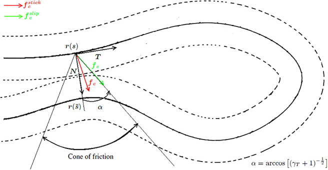
Domains of the Coulomb’s law.
The tangential sliding measurement must be carried out on the plane which is tangent to the cross-section and orthogonal to the plane
. If the self-contact during the sliding is assumed persistent, i.e.
and
. Then, we easy obtain
. And we have
3.3 Signorini-Coulomb self-contact problem
Tresca’s law has been added to contact problems when normal compressions are important. This leads to a quadratic functional minimization problem. Following Kikuchi and Oden (1988), this is based on a fixed slip potential, assumed to be known, and which does not depend on the normal stress. However, it is very sensitive and can lead to complex instability during large movements. Coulomb’s law generalizes the Tresca friction phenomenon and is able to analyze this friction of elastic rods even in case of significant displacement. He describes this threshold dependence with the intensity of normal forces. Unfortunately, also the Coulomb’s law does not admit of potential since its friction potential depends on normal compression.
The Kuhn-Tucker and the Signorini-Coulomb frictional conditions as following:
3.4 Non-uniqueness and non-existence of solutions to quasi-static frictional self-contact problem
The frictional self-contact problems as a particular case of frictional contact problems have a practical as well as a theoretical importance, a large number of algorithms for the numerical solution of the related finite element equations and inequalities as a minimization problem of potential energy have been presented in the literature. But theoretically, the quasi-static frictional self-contact problems are known to exhibit ‘unexpected’ features such as non-existence and non-uniqueness of solutions.
The typical example for the elastic energy density
, where
and
are two coercive, symmetric and positive-definite matrices in
. Such an energy functional involves shear, tension, flexure, and torsion. The constraints imposed in
are contained so that if
and
are, respectively, independent of
and
. By the kinematic equations and the Darboux vectors derivative (Chamekh et al., 2009), we are substituting the constitutive laws (4) in the balance equations (3) for obtaining the following weak form of the problem
To study the existence and uniqueness of the solution for the Signorini-Coulomb contact problems, it would be pointless to think of using classical variational methods, which may also partly explain why fixed-point theorems are widely used by many authors as in Nečas et al. (1980) and Jarušek (1983). The inapplicable fixed-point theorems for problem (11) because of the strong nonlinearity as a coupling between
and
at the level of each equation, so that we could not prove that this problem even admits a solution. Note that if we delete the coupling between
and
for example by delete the rotation
in internal force
and moment
given by (4) (which is physically not allowed actually), we obtain a purely mathematical linear problem who admits a solution demonstrable by the fixed-point theorem of Schauder for a penalized frictional self-contact force proposed and defined by
4 Numerical implementation
In the literature, the penalty and the augmented Lagrangian methods are the methods most used numerically, and which are able to respect the contact and friction conditions even on a weak form. In this paper, we are interested in these methods which are theoretically detailed in Kikuchi and Oden (1988). The penalty method authorize, firstly, a negligible self-penetration and secondly a lightweight sliding without respect the friction conditions, these permissions depend on the normal and tangential penalty parameters (Fig. 4). The penalty and the augmented Lagrangian methods were used in Wriggers and Zavarise (1997); Zavarise and Wriggers, 2000 for frictionless contact between two beams with circular sections, and recently used in Chamekh et al. (2014) and Chamekh (2015) for the numerical treatment of frictionless self-contact of a closed rod with circular sections. We will extend this study to the frictional self-contact case.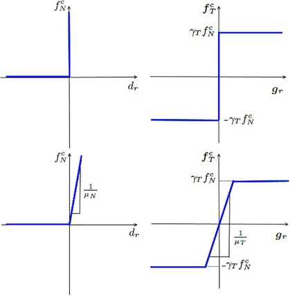
Schematic of the frictional self-contact regularizations: as the penalty parameters go to zero, the graphs (at the bottom) represent by the method of penalization coincide with the graphs (at the top) represent by the Kuhn-Tucker and friction conditions.
The principle of virtual work for the augmented Lagrangian method, it is a necessary condition for minimizing the total energy in the space of kinematically and physically admissible configurations
given by:
The self-contact and friction conditions (10) are equivalent to:
Let
be a regular configuration on
such that
,
and
verify conditions (10). First, of the condition (10b) we have
or
, suppose that
, the condition (10a) gives that
Now, suppose that
, the condition (10c) implies that
. then
so that (18a) holds. Secondly, from the friction conditions in (10) consider the case
, according to the condition (10d) we have
, then
In the case
we have
, then
Therefore
so that (18b) holds. Conversely, let
such that (18) holds. From (18a) we obtain
. Consider the first case
, then
and
which implies
. In the case
, we have
which implies that
and
. So that the Kuhn-Tucker conditions in (10) holds. Now, from (18b) suppose that
, then
which implies that
thereby (10d) holds. In the case
we obtain
because if
then
which contradicts the hypothesis. Then, the relationship (18b) can now be written:
Therefore
5 Existence and uniqueness solution of penalized frictional self-contact problem
Here we adopt the augmented Lagrangian formulation described above and the classical variational formulation of the self-contact well detailed in Chamekh et al. (2009). More precisely, the problem of finding the approximated equilibrium configurations leads to the following nonlinear approximated minimization problem
For the sake of simplicity we restrict ourselves to the cases where , and we recall that .
If the external force , then for each and , Problem (20) admits at least one solution.
A big party of this theorem is proved in Chamekh et al. (2009) for the frictionless self-contact problem based on a generalized Weierstrass minimization theorem (Kikuchi and Oden, 1988 p. 382). The first part of the energy functional is weakly lower semicontinuous and that it is coercive and the weak closure of the set is proved in Bourgat et al. (1988). It remains to prove that the penalized second part of the energy functional is weakly lower semicontinuous and that the total energy functional remains coercive after adding the nonlinear terms associated the self-contact. The frictional self-contact force is in . Then, the mapping is convex and weakly lower semicontinuous. Furthermore in Chamekh et al. (2009), it is proved that, under certain conditions we assume that they are supported here, there exist constant and such that where is the first part of the energy functional, and denotes the usual norm in if the argument is in , or if the argument is in . Since we have Therefore the functional remains coercive which ends the proof. □
6 Linearization of the virtual work of frictional self-contact forces
The integral part in (14) is the virtual work of the problem (17) that is nonlinear, to solve it, we have used the Newton-Raphson method. This method consists in solving the next linearized problem for at the iteration k with an estimate .
The frictional self-contact forces rewrites
In the following, it is necessary to calculate the directional derivatives
,
,
and
. For the directional derivative of
is given by (see Chamekh et al., 2009):
where the function F is defined by:
Using the Euler approximation of the tangential sliding velocity, we obtain:
7 Conclusions
The fusion of self-contact and friction induces a strong nonlinear problem and rich modeling, along with the nonlinearity of the modeling of a hyperelastic rod in large displacements in three-dimensional space. Theoretically, the existence and uniqueness of the solution to the problem is a major challenge. We have used the augmented Lagrangian method to address the mathematical study of the Signorini-Coulomb-self-contact problem. We have overcome the significant obstacles encountered in the implicit nature of formulations linked the use of Coulomb’s law. In addition, we have developed some formulations for the frictional self-contact problem, which can be, implemented numerically in future research.
Acknowledgment
The authors would like to thank Prof. Maher Moakher for his fruitful discussions during this work.
References
- Nonlinear Problems of Elasticity (second ed.). New York: Applied Mathematical Sciences, Springer Verlag; 2004.
- Modélisation et calcul des grands déplacements de tuyaux élastiques en flexion-torsion. J. Mécanique Théor. Appl.. 1988;7(4):379-408.
- [Google Scholar]
- Analysis of contact of elastic rods subject to large displacements. Appl. Math. Lett.. 2003;16:619-625.
- [Google Scholar]
- Modeling and numerical treatment of elastic rods with frictionless self-contact. Comput. Methods Appl. Mech. Engrgy. 2009;198(47/48):3751-3764.
- [Google Scholar]
- Stability of elastic rods with self-contact. Comput. Methods Appl. Mech. Engrgy. 2014;279:227-246.
- [Google Scholar]
- Non-linear stability criterion in numerical approximation of hyperelastic rods. Universal J. Eng. Mech.. 2015;3:45-52.
- [Google Scholar]
- Existence of solutions of Signorini problems with friction. Int. J. Eng. Sci.. 1984;22(5):567-575.
- [Google Scholar]
- Théorie des Corps Déformables. Paris: Hermann; 1909.
- Les inéquations en mécanique et physique. Paris: Dunod; 1972.
- Equilibre d’un solide élastique avec contact unilatéral et frottement de Coulomb. C.R. Acad. Sci. Paris Sér. A. 1980;290:263.
- [Google Scholar]
- On some existence and uniqueness results in contact problems with nonlocal friction. Nonlinear Anal. Theory Meth. Appl.. 1982;6:1075.
- [Google Scholar]
- Computational comparison of the bending behavior of aortic stentgrafts. J. Mech. Behav. Biomed. Mater.. 2012;5:272-282.
- [Google Scholar]
- Finite element analysis of the mechanical performances of marketed aortic stent-grafts. J. Endovasc. Ther.. 2013;20:523-535.
- [Google Scholar]
- Contact problems with bounded friction coercive case. Czechoslovak Math. J.. 1983;33(108):237-261.
- [Google Scholar]
- Anisotropic elastoplasticity for cloth, knit and hair frictional contact. ACM Trans. Graph.. 2017;36(4):14. Article 152
- [Google Scholar]
- Contact Problems in Elasticity: A Study of Variational Inequalities and Finite Element Methods. Philadelphia: SIAM; 1988.
- On friction problems with normal compliance. Nonlinear Anal. Theory Meth. Appl.. 1989;13:935-955.
- [Google Scholar]
- Geometrically exact finite element formulations for curved slender beams: Kirchhoff-Love theory vs. Simo-Reissner theory. Arch. Comput. Methods Eng. 2016
- [Google Scholar]
- An unbiased Nitsche’s formulation of large deformation frictional contact and self-contact. In: Comput. Methods Appl. Mech. Eng.. Vol 325. Elsevier; 2017. p. :265-288.
- [Google Scholar]
- Nečas, J., Jarušek, J., Haslinger, J., 1980. On the solution of the variational inequality to Signorini problem with small friction. Bolletino U.M.I., 5 17-B. pp. 796–811.
- Contact problems in elastostatics with non-local friction law. J. Appl. Mech.. 1983;50:67-76.
- [Google Scholar]
- Models and computational methods for dynamic friction phenomena. Comput. Methods Appl. Mech. Eng.. 1985;50(1–3):527-634.
- [Google Scholar]
- On finite deformations of space curved beams. J. Appl. Math. Phys.. 1981;32:734-744.
- [Google Scholar]
- A uniqueness criterion for the Signorini problem with Coulomb friction. SIAM J. Math. Anal.. 2006;38(2):452-467.
- [Google Scholar]
- On the dynamics in space of rods undergoing large motions – a geometrically exact approach. Comput. Methods Appl. Mech. Eng.. 1988;66(2):125-161.
- [Google Scholar]
- Instability and self-contact phenomena in the writhing of clamped rods. Int. J. Mech. Sci.. 2003;45:161.
- [Google Scholar]
- On contact between three-dimensional beams undergoing large deflection. Commun. Numer. Methods Eng.. 1997;13:429-438.
- [Google Scholar]
- Contact with friction between beams in 3-d space. Int. J. Numer. Meth. Eng.. 2000;49:977-1006.
- [Google Scholar]


