

Translate this page into:
“Forecasting particulate matter concentrations by combining statistical models”
⁎Corresponding author. mtzateroglu@cu.edu.tr (Mine Tulin Zateroglu)
-
Received: ,
Accepted: ,
This article was originally published by Elsevier and was migrated to Scientific Scholar after the change of Publisher.
Abstract
Air pollutants have adverse effects on human health and play significant roles in urban planning and specifying air quality ranges. Atmospheric particulate matter is one of the criteria air pollutants that may have a dominant effect on air pollution. The present analysis was made using data collected over five years (2011–2015) in an urban area. Air pollutant concentrations and climate data are analyzed using four models: a multiple linear regression model, a principle component regression model, a logarithmic architecture, a principle component regression model with the variables that only have the highest factor loadings in each principal component. Thus, the proposed model combines both methods the multiple linear regression and the principal component analysis to obtain clearer and more reliable predictions. The prediction model’s accuracy has been verified operating several performance indicators, which revealed acceptable values, demonstrating that the proposed model can be used to predict pollutant concentrations. According to statistical indicators (RMSE, NMSE, CV, FB and IOA), the best prediction models were Model 3 for winter (0.06, 0.001, 0.03, −0.000, and 0.69), Model 4 for spring (0.08, 0.002, 0.04, −0.019, and 0.99), Model1 for summer (3.41, 0.005, 0.07, 0.000, and 0.98), and Model 2 for autumn (11.71, 0.018, 0.13, −0.000, and 0.57). In addition, Model2 generally gave appropirate values for all seasons and can be used as a common model. Finally, combined models based on principal component analysis and multiple linear regression outperformed models with only multiple linear regression in terms of error.
Keywords
Particulate matter
Climate parameters
Regression
Principal Component Analysis

1 Introduction
Urban air pollution analysis has a key role in urban planning and determining the air quality index. Air pollution induced by particulate matter (PM) has been studied as a well-known problem in many areas around the world. Because of its damaging effects on the environment, atmosphere, and human health, it is an important topic in urban regions (Deryugina et al., 2019; Barnaba et al., 2022; Marques et al., 2022; Farahani et al., 2022, Sharma et al., 2022; Cho et al., 2022; Kim et al., 2022; Santibanez-Andrade et al., 2022). PM in cities may originate from dust, smoke particles, metals, etc. PM10 is particulate matter in the atmosphere that is characterized by a particle diameter of 10 µm or less, which consists of liquids, solids, or mixtures of both. There are various sources of PM10, e.g., traffic density, fuel combustion, sea salt, dust, inversion, etc. The different forms of PM generally include dust, smoke, and soot, which originate from natural and anthropogenic sources such as industrial and combustion activities (Kassomenos et al., 2014). PM10 has adverse effects on the environment, particularly in agriculture, and on human health, for instance, causing respiratory diseases, lung cancer, and cardiovascular system damage (Santibanez-Andrade et al., 2022). Therefore, an increase in PM makes urban air quality worse. The impact of PM10 is also greatly affected by seasonal changes and atmospheric conditions because meteorological parameters are related to each other in the atmosphere (Latif et al., 2014; Zateroglu, 2021a). Air pollutants are tied to climate elements and various interactions in urban atmospheric environments (Turnock et al., 2015; Zateroglu, 2021b, 2021c; Cipoli, et al., 2023). Furthermore, meteorological variables can affect the concentrations of air pollutants in the atmospheric periphery (Galindo et al., 2011; Gvozdić et al., 2011; Zateroglu, 2022). Accordingly, it is necessary to understand the meteorological parameters’ impact on the PM to reduce their influences and develop sustainable management strategies. Furthermore, Pasquill–Gifford–Turner (PGT) protocol denotes the relations between climate parameters and air pollutants. A PGT scheme can be used to estimate the horizontal and vertical dispersion of a plume in air pollution models, i.e., Gaussian models (Venkatram, 1996). These models consider stable atmospheric conditions, i.e., solar radiation, cloudiness, constant wind speed, and vertical temperature gradient.
The concentrations of air pollutants are related to inversion, higher pressure system, higher relative humidity, colder air temperatures, lower wind speed, and lower precipitation (Tayanç and Berçin, 2007). Especially in winter period, due to the cold air close the surface, intensive inversion is formed, resulting in an increase in the concentrations of air pollutants (Wanner and Hertig, 1984). The parameters, precipitation and wind speed have influences on the concentrations of air pollutant by cleaning and dispersing in the atmospheric environment. Wind speed defines the dispersion and horizontal transportation of air pollutants. High level of wind speed diffuse the concentrations of air pollutants whereas low level produce haze episodes. However, depending on wind direction and topography, high level of wind speed may contribute the deposition of pollutant concentrations rather than disperse them. Furthermore, high wind speed can result in enhanced evaporation ratio of air pollutants and reduced air pollutant concentrations. Low level of particulate matter contains high level evaporation. Moreover, in the conditions with high relative humidity, water vapor in the humid air keeps the particles suspended in the atmospheric periphery, causing the particulate matter concentration to reduce (Barmpadimos et al., 2011). High level of air temperatures result in high air pollutant dispersion (Verma and Desai, 2008). Furthermore, air pollutants’ concentrations can scatter and reflect solar radiation, ultimately decreasing the surface temperature. Meteorological measurements contribute to evaluating the influences of meteorological parameters on environment and air quality (Falocchi et al., 2020).
Estimating air pollutant quantity is required for air quality regulations. This current study can provide insight into the behaviors of air pollutants and help in reducing their impacts. Various statistical methods have been performed on meteorological studies to predict PM concentrations (Ceylan and Bulkan, 2018; Özdemir and Taner, 2014; Ramli et al., 2023). Multiple linear regression method is one of the most preferred techniques and has been used for years (Zaman et al., 2017). Multiple linear regression (MLR), principal component analysis (PCA), and combined models have been applied to estimate meteorological parameters (Ul-Saufie et al., 2013). Since the air pollutants’ deposition, dispersion and transportation are affected by regional climate situations, climate elements can be used to estimate and control the emissions of air pollutants. However, the estimations need to be optimized for different seasonal periods and the overall performance of the constructed models can be improved by interpreting more datasets. Therefore, this paper analyzes the appropriate mathematical models using MLR and PCA for predicting the concentration of PM10 in an urban area in Turkey, using data compiled over five years. All simulations are used to estimate the particulate matter concentration, utilizing the climate parameters, the sulfur dioxide concentration, to model the situation when particulate matter is not measured. The main aim of this study is to determine the important meteorological parameters in the estimation of PM10 concentration.
2 Study area and data
The present work was conducted in Denizli province, situated in western part of Turkey. Denizli province, with an area of 11,868 km2, altitude of 425 m, is located between 37°12′ and 38° 12′ northern latitudes and 28°30′ and 29°30′ east longitudes, in the Anatolian peninsula, at the intersection of the Aegean-Central Anatolia and Mediterranean Regions (Fig. 1). Furthermore, its climate varies because of the geographical diversity. Since the mountains in Denizli mostly extend perpendicular to the sea, they are open to the winds coming from the sea.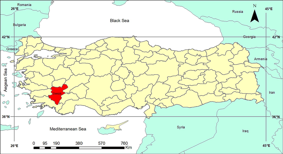
Turkey and the location of Denizli Province.
In most of the known climate classification methods, Denizli province is in a climate class that is semi-arid and less humid, cool in winters, hot in summers. In summer, when the Basra Low Pressure Center occurs in the province, the temperatures rise considerably. According to long-term records, the average annual precipitation is 568.7 mm. The average annual temperature is 16.2 °C. The average number of rainy days is 91. The prevailing wind direction is northwest (NW). The classification of the monthly distiribution of each dataset is presented in Table 1 shown in Appendix A. Denizli has a large-scale cotton-based textile industry, rolling mills, metal industry, food industry, cable and construction materials industry, and travertine and marble industry. Fossil fuels, especially coal, are used in industrial plants and domestic heating. The main sources of pollution are fossil fuel consumption for domestic heating and industrial activities, vehicle emissions, ground dust, and leaks in Denizli. Because of the low amount of precipitation in summer, dust emission by wind may have increased.
Month
PM10
SO2
SD
CLD
RH
WS
PREC
EVP
PRES
MINT
MAXT
JAN
143.35
165.49
117.19
4.62
70.60
1.04
64.93
NA
968.23
−3.84
17.59
FEB
112.26
135.74
127.70
4.87
67.83
1.27
75.73
NA
966.94
−3.87
19.68
MAR
86.15
101.17
181.60
4.40
63.44
1.21
66.12
NA
965.50
−0.33
24.30
APR
65.13
62.29
204.69
4.62
60.92
1.14
60.95
86.83
963.85
3.67
29.40
MAY
51.50
45.07
287.29
3.43
54.10
1.16
40.83
146.22
963.81
8.13
33.73
JUN
46.82
36.94
336.24
2.00
45.93
1.32
25.15
194.65
962.66
13.46
38.06
JUL
53.38
35.54
365.85
1.19
43.60
1.34
21.49
231.12
960.29
17.51
39.86
AUG
50.76
37.34
335.24
1.06
46.18
1.18
11.95
206.20
961.00
17.48
39.70
SEP
54.87
44.90
269.99
1.51
51.60
1.01
14.11
139.47
964.30
11.88
36.46
OCT
70.19
43.77
201.30
2.98
60.46
0.90
32.65
84.64
967.21
6.19
31.20
NOV
120.76
105.09
144.05
3.93
67.11
1.01
65.38
39.18
968.41
0.85
24.93
DEC
136.41
138.08
98.08
5.20
72.56
1.06
87.68
NA
968.13
−2.80
18.98
3 Methods
To measure PM10 concentrations, a Beta beam attenuation monitor is used in the air quality monitoring station which is located in residential area. The daily mean data was recorded for five years (2011 to 2015) at the monitoring station in the studied province. For estimation and subsequent verification of the analysis, the daily average meteorological parameters, such as particulate matter, PM10 (µg/m3), sulfur dioxide, SO2 (µg/m3), relative humidity, RH (%), cloudiness, CLD (0–8), sunshine duration, SD (hour), maximum air temperature, MAXT (oC), minimum air temperature, MINT (oC), air pressure, PRES (hPa), precipitation amount, PREC (mm), wind speed, WS (m/s), and evaporation, EVP (mm), were obtained and organized by season. All data were grouped into four seasons, namely winter (December to January), spring (March to May), summer (June to August), and autumn (September to November). The data for climate parameters were provided by the Turkish State Meteorological Service while the data for air pollutants were provided by the Ministry of Environment and Urbanism (MEU, 2023). There are four models used for forecasting of daily PM10. These models as explained in Appendix B are namely multiple linear regression (Model1), principle component regression (Model2), logarithmic architecture (Model3), principle component regression model with the variables that only have the highest factor loadings in each principal component (Model4). The MLR method was used to construct the four models in the estimation. For training aims, data for a period of 2011–2014 have been utilized as input variables to the four models. Then, the constructed models have been used to estimate daily PM10 of the next year 2015. Furthermore, the estimated values of PM10 obtained from models have been compared with measured concentration values of PM10 of the year 2015 through the statistical indicators. Table 2 shows the performance indexes, which reveal the success of the estimated models (Appendix B). Notably, Ek is the predicted value, Mk is the observed value,
is the average value of the observed values, and n is the number of observations.
Statistical Indicator
Formula
Ideal Value
Root Mean Square Error
0
Coefficient of Variation
0
Fractional Bias
0
Normalized Mean Square Error
0
Index of Aggrement
1
In the present work, SPSS (Statistical Package for Social Science) software has been used for the statistical evaluations. At the beginning of the analysis, the missing values existing in the dataset were fulfilled by employing the expectation maximization method. To specify the distribution of meteorological variables and concentrations of air pollutants, one-sample Kolmogorov–Smirnov test has been applied to dataset.
4 Results and discussion
Four statistical structures, Model1, Model2, Model3, and Model4, have been operated to estimate PM10 during 2011–2014. The daily PM10 has been predicted using measured climate elements and SO2 in all the four seasonal periods. The parameters of interest are climatological variables i.e., RH, CLD, SD, PRES, WS, EVP, PREC, MINT, MAXT, and air pollutants i.e., PM10 and SO2. The variation of the values for each variable differed depending on the seasons.
Fig. 2 shows the monthly mean variations of meteorological parameters used in this study for normalized values from January (JAN) to December (DEC). As seen in Fig. 2, particulate matter concentration is positively associated with the sulfur dioxide, relative humidity, cloudiness, precipitation, pressure, whereas negatively with sunshine duration, wind speed, evaporation, and air temperatures, with exceptional cases. Galindo et al. determined that the particulate matter concentration was inversely related to wind speed (Galindo et al., 2011). In addition, the highest PM10 concentrations were obtained in the period from November to March. Similar result was presented in another research for December to March (Silva et al., 2017; Cordova et al., 2021). High values are associated with winter season when fossil fuel combustion increases for domestic heating (Ceylan and Bulkan, 2018).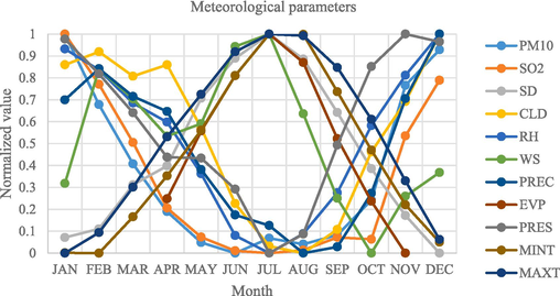
Monthly mean variations of meteorological parameters.
The results of varimax rotation are shown in Table 3(a-d). Loadings of climate variables and sulfur dioxide pollutant for any component as bold are indicated for varimax rotation seasonally.
(a)
(b)
WINTER
SPRING
PC1
PC2
PC1
PC2
PC3
PC4
SD
−0.82
0.35
SD
−0.86
0.09
0.15
0.30
CLD
0.73
−0.07
CLD
0.78
−0.29
0.10
0.24
RH
0.73
0.60
RH
0.65
−0.32
−0.17
0.55
WS
0.45
−0.64
WS
0.07
0.95
0.07
−0.06
PREC
0.79
−0.32
PREC
0.73
0.06
−0.24
0.23
PRES
−0.86
0.39
EVP
−0.38
0.79
0.17
−0.06
MINT
0.55
0.08
PRES
−0.61
−0.37
−0.59
−0.22
MAXT
0.15
−0.86
MINT
−0.08
0.11
0.86
−0.03
SO2
−0.03
0.73
MAXT
−0.28
0.03
0.64
−0.41
SO2
0.05
−0.05
−0.09
0.94
Eigenvalue
4.09
1.96
Eigenvalue
3.66
1.97
1.31
1.11
% of Variance
45.5
21.8
% of Variance
36.6
19.7
13.1
11.1
Cumulative %
45.5
67.3
Cumulative %
36.6
56.3
69.4
80.5
(c)
(d)
SUMMER
AUTUMN
PC1
PC2
PC3
1
2
3
4
5
SD
0.02
0.77
0.38
SD
0.20
−0.11
−0.22
0.85
−0.04
CLD
−0.02
−0.84
0.21
CLD
0.09
0.22
0.83
0.02
0.07
RH
−0.78
0.08
0.37
RH
0.85
0.04
0.17
−0.23
−0.31
WS
0.70
0.06
−0.22
WS
−0.47
0.54
0.15
−0.23
0.54
PREC
−0.52
−0.54
−0.30
PREC
−0.13
−0.05
0.79
−0.16
0.13
EVP
0.87
0.14
0.07
EVP
0.03
−0.00
0.16
−0.01
0.89
PRES
−0.52
0.63
0.15
PRES
−0.14
−0.91
−0.09
0.07
−0.21
MINT
0.82
−0.01
−0.41
MINT
−0.33
0.81
0.06
−0.04
−0.29
MAXT
0.90
−0.23
0.15
MAXT
−0.46
−0.03
0.09
0.79
−0.00
SO2
−0.19
0.12
0.93
SO2
0.85
−0.19
−0.19
0.11
0.30
Eigenvalue
4.11
2.25
1.16
Eigenvalue
2.77
1.97
1.39
1.15
1.06
% of Variance
41.1
22.5
11.6
% of Variance
27.7
19.7
13.9
11.5
10.6
Cumulative %
41.1
63.6
75.2
Cumulative %
27.7
47.4
61.3
72.8
83.4
The seasoned data analysis finding indicated that winter had two PCs that eigenvalues bigger than 1 (4.09 and 1.96) while spring, summer and autumn had four, three, and five PCs, respectively. Additionally, the cumulative percentages for winter, spring, summer, and autumn were 67.3 %, 80.5 %, 75.2 %, 83.4 %, respectively. The variance percentages were 45.45 % for PC1 (SD, CLD, RH, PREC, PRES, MINT) and 21.82 % for PC2 (WS, MAXT, SO2) in winter; 36.6 % for PC1 (SD, CLD, RH, PREC, PRES), 19.7 % for PC2 (WS, EVP), 13.1 % for PC3 (MINT, MAXT) and 11.1 % for PC4 (SO2) in spring; 41.1 % for PC1 (RH, WS, EVP, MINT, MAXT), 22.5 % for PC2 (SD, CLD, PREC, PRES) and 11.6 % for PC3 (SO2) in summer; 27.7 % for PC1 (RH, SO2), 19.7 % for PC2 (WS, PRES, MINT), 13.9 % for PC3 (CLD, PREC), 11.5 % for PC4 (SD, MAXT), and 10.6 % for PC5 (EVP) in autumn. In winter, PC1 and PC2 explained 67.3 % of the variance, with decreasing sunshine duration, maximum air temperature, low pressure level and wind speed favoring increased cloudiness, relative humidity, precipitation, minimum air temperature, and sulfur dioxide, increasing PM10. In spring, four principal components explained 80.5 % of the variance, with higher cloudiness, relative humidity, precipitation, wind speed, evaporation, air temperatures, and sulfur dioxide favoring higher PM10 dispersion. In summer, principal components PC1, PC2, and PC3 explained 75.2 % of the variance with descending cloudiness, relative humidity, precipitation favoring increased sunshine duration, wind flows, evaporation, pressure, sulfur dioxide, and temperatures, enhancing PM10. In autumn, five principal components explained 83.4 % of the variance with decreasing pressure favoring increased relative humidity, sulfur dioxide, sunshine duration, cloudiness, wind speed, precipitation, temperatures and evaporation, increasing PM10.
The strongly loaded variables for PCs are pressure and maximum temperature in winter; sunshine duration, wind speed, minimum temperature, and sulfur dioxide in spring; maximum temperature, cloudiness, and sulfur dioxide in summer; sulfur dioxide, relative humidity, pressure, cloudiness, sunshine duration, and evaporation in autumn.
Furthermore, sunshine duration and pressure had a negative correlation in PC1, whereas cloudiness, relative humidity, precipitation, and minimum temperature had a positive relation in winter. The maximum temperature and wind speed had a negative correlation, but sulfur dioxide was positively correlated in PC2. The relations for all PCs in the other seasons were positive for precipitation, evaporation, and sulfur dioxide, negative for the sunshine duration, and both positive and negative for cloudiness, relative humidity, precipitation, wind speed, and pressure. Meteorological parameters, such as an increase in air temperature and humidity and a decrease in wind speed, contribute to greater concentrations of PM10 (Kassomenos et al., 2014; Barmpadimos et al., 2011).
The scores of principal components have been calculated as referred in Eq. (4). The parameters’ standardized values have been multiplied by standardized weights. The scores obtained in PCA analysis have been employed as explanatory parameters in MLR analysis for PCR models. In MLR analysis with stepwise regression method, score variables with statistically significant (95 % confidence interval) values were chosen and non-significant values were excluded from the estimation model for PM10.
MLR method is used in all the four models. The results of MLR analysis, i.e., stepwise regression, are shown in Table 4. According to the findings, emprical models were constructed for season-based analysis. Four prediction models were obtained for each season. In winter, low levels of relative humidity, high levels of pressure, and maximum air temperature are crucial inputs, as shown in Models 1 and 4. Particulate matter concentration is inversely related to relative humidity (Reategui-Romero et al., 2021). In spring, the maximum air temperature was selected by stepwise regression in Model 1, whereas high sunshine duration, wind speed, minimum temperature, and low sulfur dioxide were selected in the Model 4. The concentration of air pollutant is positively related to sunshine duration (Barmpadimos et al., 2011). Low levels of sulfur dioxide and maximum air temperature, and high levels of cloudiness were significant explanatory variables in summer. In autumn, high cloudiness, pressure, and evaporation where important, whereas low sulfur dioxide and sunshine duration were chosen as important variables in Model 1. Cloudiness, gradient of vertical air-temperature, solar radiation, and wind speed are closely related to dispersion of air pollutant concentration via the PGT scheme. Solar radiation is strongly related to sunshine duration based on the Angström–Prescott formula; therefore, sunshine duration is associated with air pollutant concentrations. Mutual effects between climate variables and air pollutants exhibit a decrement or increment in air pollutant concentrations.
Term
Model No
Model equation
WINTER
1
PM10 = 353.4 – 3.2 * RH
2
PM10 = 131.6 – 12.2 * SCORE1
3
logPM10 = 2.1 – 0.04 * SCORE1
4
logPM10 = − 24.1 + 0.03 * PRES + 0.02 * MAXT
SPRING
1
PM10 = − 22.2 + 3.1 * MAXT
2
PM10 = 68.5 – 3.5 * SCORE1 + 0.8 * SCORE2 + 1.3 * SCORE3 − 3.1 * SCORE4
3
logPM10 = 1.8 – 0.02 * SCORE1 + 0.001 * SCORE2 + 0.009 * SCORE3 − 0.02 * SCORE4
4
logPM10 = 1.6 + 0.001 * SD + 0.03 * WS + 0.001 * MINT − 0.0004 * SO2
SUMMER
1
PM10 = 77.7 – 0.8 * SO2
2
PM10 = 48.9 – 10.3 * SCORE3
3
logPM10 = 1.7 – 0.08 * SCORE3
4
logPM10 = 1.95 – 0.001 * MAXT + 0.004 * CLD − 0.006 * SO2
AUTUMN
1
PM10 = 50.7 + 12.97 * CLD
2
PM10 = 87.7 + 6.2 * SCORE3
3
logPM10 = 1.9 + 0.03 * SCORE3
4
logPM10 = − 9.8 – 0.001 * SO2 + 0.01 * PRES + 0.05 * CLD − 0.001 * SD + 0.001 * EVP
The visual of the observed and predicted values for seasonal data is indicated in Fig. 3. Since the PM10 pollutant has an adverse effect on the urban climate and human health, in this study the particulate matter concentration has been estimated starting from the SO2 concentration, that is commonly measured. The SO2 pollutant and climate parameters were utilized as input variables in the simulations to estimate the concentration of PM10.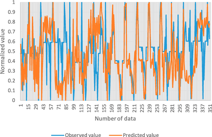
Observed and predicted values.
The performance evaluation of predicted PM10 values was presented in Table 5 via four statistical models. The verification results, presented in Table 5, reveal that models for PCR performed better than MLR in respect to error. Furthermore, the best prediction models were Model 3 for winter, Model 4 for spring, Model1 for summer, and Model 2 for autumn. Several reseaerchers have found IOA values such as 0.80–0.89 (Grivas and Cholokou, 2006), 0.86 (Papanastasiou et al., 2007), approximately 0.857–0.9257 (Sfetsos and Vlachogiannis, 2010), 0.5928–0.9278 (Ul-Saufie et al., 2013). The obtained results of IOA in present study (0.69 for winter, 0.99 for spring, 0.98 for summer, 0.57 for autumn) is close to previous studies. When considering PCR and MLR as in this study, statististical indices are higher utilizing PCR (Sousa et al., 2007).
Term
Model No
RMSE
NMSE
CV
FB
IOA
Winter
1
17.64
0.018
0.13
0.000
0.65
2
17.49
0.018
0.13
0.000
0.66
3
0.06
0.001
0.03
−0.000
0.69
4
0.31
0.019
0.15
0.136
0.23
Spring
1
10.89
0.025
0.16
−0.000
0.50
2
10.94
0.025
0.16
0.000
0.52
3
0.07
0.001
0.04
−0.000
0.56
4
0.08
0.002
0.04
0.019
0.99
Summer
1
3.41
0.005
0.07
0.000
0.98
2
5.25
0.012
0.11
−0.000
0.94
3
0.05
0.001
0.03
0.000
0.91
4
0.04
0.001
0.02
0.005
0.96
Autumn
1
11.77
0.018
0.13
0.000
0.56
2
11.71
0.018
0.13
−0.000
0.57
3
0.06
0.001
0.03
0.000
0.53
4
0.22
0.014
0.11
−0.115
0.30
5 Conclusion
This study focuses on the predicting of daily PM10 concentration in urban province Denizli. PM is one of the air pollutants that have an important effect on urban air quality and human health. This work aimed to determine the variables that have crucial effects on PM10 estimation by comparing different models such as a multiple linear regression model, a principal component regression model, a logarithmic model, a principal component regression model with the variables that only have the highest factor loadings in each principal component. The data of air pollutants and climate variables were categorized by season. For each season, four models mentioned above were established to forecast the concentration of PM10 and determine the most accurate prediction model. The performance evaluations of all the four models for each season indicated that prediction success varies because of the changing influence of variables. The results show that error values are generally close to each other for every season when using Model 1 and Model 2. Additionally, Model 3 and Model 4, with base-ten logarithms, gave different results for the various seasons, except in summer, which exhibited similar values for each model. Model 3 provides more suitable values in comparison with Model 4.
Using principal components in the prediction effectively reduced multicollinearity in the regression models by providing specification of the suitable explanatory variables. Comparing the success of the models, the PCR models with varimax rotation give more reliable results than the others. Hence, this Model2 can be used for PM10 predicting in other urban areas of Turkey. The increase or decrease in the levels of climatological parameters, used in this study, has an impact on the levels of particulate matter concentration in each season. Especially air temperature, wind speed, and precipitation cause variations on the quantity of particulate matter concentration, accumulation in the atmosphere and its transport. Low grades of precipitation, air temperature, and wind speed and high grades of relative humidity and pressure produce high grades of particulate matter concentrations. High level of pressure blocks the air flow from the surrounding areas from entering into the region. Low level of wind speed does not disperse particulate matter concentrations, resulting in an increase in air pollution. Further, some elements, e.g. fossil fuel combustion, inversion, industrial emissions, motor vehicles, increment in energy usage with population growth, topography, atmospheric oscillations have effects on the level of particulate matter concentration.
Finally, it can be finalized that in the analogous conditions, the Model2 can be used for daily particulate matter estimating in any urban province. Accurate predictions of PM concentrations can help clarify the air quality levels and enhance public awareness, allowing for the development of more useful policies and precautions in urban areas. As next study, it is aimed to develop new prediction models through the implementation of geostatistical models and machine learning methods to evaluate the success in the models.
Declaration of competing interest
The authors declare that they have no known competing financial interests or personal relationships that could have appeared to influence the work reported in this paper.
References
- Influence of meteorology on PM10 trends and variability in Switzerland from 1991–2008. Atmos. Chem. Phys.. 2011;11:1813-1835.
- [Google Scholar]
- Multiannual assessment of the desert dust impact on air quality in Italy combining PM10 data with physics-based and geostatistical models. Environ. Int.. 2022;163:107204
- [Google Scholar]
- Forecasting PM10 levels using ANN and MLR: A case study for Sakarya City. Global NEST J.. 2018;20(2):281-290.
- [Google Scholar]
- The influence of atmospheric blocking on regional PM10 aerosol transport to South Korea during February-March of 2019. Atmos. Environ.. 2022;277:119056
- [Google Scholar]
- Cipoli, Y. A., Alves, C., Rapuano, M., Evtyugina, M., Rienda, I.C., Kováts, N., Vicente, A., Giardi, F., Furst, L., Nunes, T., Feliciano, M., 2023. Nighttime–daytime PM10 source apportionment and toxicity in a remoteness inland city of the Iberian Peninsula. Atmospheric Environment, 303, 119771, ISSN 1352-2310.
- Air quality assessmentand pollution forecasting using artificial neural networks in metropolitan Lima-Peru. Sci. Rep.. 2021;11:1-19.
- [Google Scholar]
- The Mortality and Medical Costs of Air Pollution: Evidence from Changes in Wind Direction. Am. Econ. Rev.. 2019;109:4178-4219.
- [Google Scholar]
- A dataset of tracer concentrations and meteorological observations from the Bolzano Tracer EXperiment (BTEX) to characterize pollutant dispersion processes in an Alpine valley. Earth Syst. Sci. Data. 2020;12:277-291.
- [Google Scholar]
- Tailpipe and Nontailpipe Emission Factors and Source Contributions of PM10 on Major Freeways in the Los Angeles Basin. Environ. Sci. Technol.. 2022;56(11):7029-7039.
- [Google Scholar]
- The influence of meteorology on particulate matter concentrations at an urban Mediterranean location. Water Air Soil Pollut.. 2011;215:365-372.
- [Google Scholar]
- Articial neural networks models for prediction of PM10 hourly concentrations in the Greater Area of Athens. Greece. Atmospheric Environ.. 2006;40(7):1216-1229.
- [Google Scholar]
- Influence of meteorological factors NO2, SO2, CO and PM10 on the concentration of O3 in the urban atmosphere of eastern Croatia. Environ Model Assess. 2011;16(5):491-501.
- [Google Scholar]
- Applied Multivariete Statistical Analysis. Englewood Cliffs, USA: Prentice-Hall Inc.; 1982. p. :590.
- Study of PM 10 and PM 2.5 levels in three European cities: analysis of intra and inter urban variations. Atmos Environ. 2014;87:153-163.
- [Google Scholar]
- Short-term prediction of particulate matter (PM10 and PM2.5) in Seoul, South Korea using tree-based machine learning algorithms. Atmospheric. Pollut. Res.. 2022;13(10):101547
- [Google Scholar]
- Long term assessment of air quality from a background station on the Malaysian Peninsula. Sci Total Environ. 2014;482–483:336-348.
- [Google Scholar]
- Long-term exposure to PM10 above WHO guidelines exacerbates COVID-19 severity and mortality. Environ. Int.. 2022;158:106930
- [Google Scholar]
- MEU, 2023. The Ministry of Environment and Urbanisation, http://www.sim.csb.gov.tr.
- Impacts of Meteorological Factors on PM10: Artificial Neural Networks (ANN) and Multiple Linear Regression (MLR) Approaches. Environ. Forensic. 2014;15(4):329-336.
- [Google Scholar]
- Development and assessment of neural network and multiple regression models in order to predict PM10 levels in a medium-sized Mediterranean city. Water Air Soil Pollut.. 2007;182:325-334.
- [Google Scholar]
- Performance of Bayesian Model Averaging (BMA) for Short-Term Prediction of PM10 Concentration in the Peninsular Malaysia. Atmos.. 2023;14:311.
- [CrossRef] [Google Scholar]
- Reategui-Romero, W., Zaldivar-Alvarez, W.F., Pacsi–Valdivia, Sánchez-Ccoyllo, O.R., García-Rivero, A.E., Moya–Alvarez, A., 2021. Behavior of the Average Concentrations As Well As Their PM10 and PM2.5 Variability in the Metropolitan Area of Lima, Peru: Case study February and July 2016. Int. J. Environ. Sci. Dev., 12, 204–213.
- Particulate matter (PM10) destabilizes mitotic spindle through downregulation of SETD2 in A549 lung cancer cells. Chemosphere. 2022;295:133900
- [Google Scholar]
- Sfetsos, A., Vlachogiannis, D., 2010. A new methodology development for the regulatory forecasting of PM10. Application in the Greater Athens Area, Greece. Atmospheric Environ., 44(26), 3159-3172.
- Novel hybrid deep learning model for satellite based PM10 forecasting in the most polluted Australian hotspots. Atmos. Environ.. 2022;279:119111
- [Google Scholar]
- Particulate matter levels in a South American megacity: The metropolitan areaof Lima-Callao. Peru. Environ. Monit. Assess.. 2017;189:635.
- [Google Scholar]
- Multiple Linear Regression and artificial neural networks based on principal components to predict ozone concentrations. Environ. Model. Softw.. 2007;22:97-103.
- [Google Scholar]
- Applied Multivariate Statistics for the Social Science. New Jersey, USA: Hillsdale; 1986. p. :515.
- SO2 modeling in İzmit Gulf, Turkey during the winter of 1997: 3 cases. Environ. Model. Assess.. 2007;12:119-129.
- [Google Scholar]
- Modelled and observed changes in aerosols and surface solar radiation over Europe between 1960–2009. Atmos. Chem. Phys.. 2015;15:9477-9500.
- [Google Scholar]
- Future daily PM10 concentrations prediction by combining regression models and feedforward backpropagation models with principle component analysis (PCA) Atmos Environ. 2013;77:621-630.
- [Google Scholar]
- An examination of the Pasquill-Gifford-Turner dispersion scheme. Atmos. Environ.. 1996;30(8):1283-1290.
- [Google Scholar]
- Effect of Meteorological Conditions on Air Pollution of Surat City. J. Int. Environm. Appl. Sci.. 2008;3(5):358-367.
- [Google Scholar]
- Studies of urban climates and air pollution in Switzerland. J. Clim. App. Meteorol.. 1984;23:1614-1625.
- [Google Scholar]
- Estimating particulate matter using satellite based aerosol optical depth and meteorological variables in Malaysia. Atmos. Res.. 2017;193:142-162.
- [Google Scholar]
- Statistical Models For Sunshine Duration Related To Precipitation and Relative Humidity. European Journal of Science and Technology. 2021;29:208-213.
- [CrossRef] [Google Scholar]
- Assessment of the Effects of Air Pollution Parameters on Sunshine Duration in Six Cities in Turkey. Fresen. Environ. Bull.. 2021;30(02A):2251-2269.
- [Google Scholar]
- The Role of Climate Factors on Air Pollutants (PM10 and SO2) Fresen. Environ. Bull.. 2021;30(11):12029-12036.
- [Google Scholar]
- Modelling the Air Quality Index for Bolu, Turkey. Carpathian J. Earth Environm. Sci.. 2022;17(1):119-130.
- [CrossRef] [Google Scholar]
Appendix A
Observed values of monthly distributions.
Table 1 Colormap of monthly distributions.
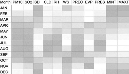
Classification of monthly distribution of winter, spring, summer, and autumn seasons is also shown as a colormap. The magnitude of the values for each dataset is represented as color. Table 1 indicates the monthly variations of the meteorological parameters used in present study. The parameters of interest are climatological variables such as RH, CLD, SD, PRES, EVP, PREC, MINT, MAXT, WS, and air pollutants i.e., PM10 and SO2. In Table 1, the values of EVP are coded as NA (not available) for winter because lack of data. The variation of the values for each variable differed depending on the months.
Appendix B
The root mean square error (RMSE), coefficient of variation (CV, the coefficient of variation of RMSE or normalized root mean square error, normalized over the mean of the original data), fractional bias (FB), index of agreement (IOA) and normalized mean square error (NMSE) have been computed to identify the model compatibility. The IOA rate changes from 0 to 1 and indicates whether the prediction is free of error. The RMSE is a gauge as diference between forecasted and observed value. An NMSE value of 0 is ideal, but small values also represent model suitability, representing a measure of scatter in the data. FB represents the measure of mean bias for the values and its range varies from the − 2 (underestimation) to + 2 (overestimation), and 0 is ideal. Model 1
MLR is a statistical method used to estimate the changeability between the variables of response and explanation. In this analysis, PM is the response variable, and sulfur dioxide and meteorological parameters are the explanatory variables. The contributions of explanatory variables to PM are computed as percentages via this technique. MLR involves one response variable and two or more explanatory parameters. The relation between explanatory variables and response variable acquired from MLR examination is determined as a mathematical form as in Eq. (1),
where Ɛ indicates the predicted error term, Y determines response parameter, X1, X2, ……, Xr denote independent parameters, ao is contant, and a1, a2, ……., ar define regression coefficients. To reduce the error parameter, the least squares method is employed for the prediction of the values of constant and coefficients in the regression model by applying the coefficient matrix a with dimensions of r x 1. Coefficient matrix a is determined using the formula a = (XTX)-1(XTY). The term r demonstrates the explanatory variables’ number, and n shows the measurements’ number. Y is measured values matrix of the response variable with dimensions of n x 1, X is the observed values matrix of explanatory variables with dimensions of n x r. In addition, XT defines X’s transpose. A distribution of F is used for expressing the relation between the response and explanatory variables, and a t-test is employed for clarifying the significance of the constants and coefficients. The model conformity is specified in terms of estimation error and a determination coefficient. The estimated models were considered significant for confidence intervals over 95 %.
To forecast the PM10 concentrations, Model1 with MLR method was examined at first. In Model1 with MLR, all data such as climate variables i.e., RH, CLD, SD, MAXT, MINT, PRES, EVP, PREC, WS, and criteria air pollutant i.e., sulfur dioxide, were used as explanatory variables to forecast the response variable, PM10. Model 2
In this study, PCA was implemented on the meteorological parameters and sulfur dioxide data to assess their significance and determine their correlation. The variables’ selected principal component scores have been employed as independent variables in regression analysis models to forecast the concentration of PM. Bartlett’s sphericity test (χ2 is calculated by the formula k(k-1)/2) has been employed to certify whether PCA is suitable for examining the data (Stevens, 1986). Further, the Kaiser Meyer Olkin (KMO) scale, which is considered appropriate for values greater than 0.5, was used for assessing the suitability of the observations. The eigenvalues of the principal components were obtained by applying Eq. (2) (Johnson and Wichern, 1982),
The components obtained from the analysis should be rotated by varimax rotation, which is commonly used, to provide more clear relationships between the original input parameters and generated principal components. By the varimax technique, any variable can be distinguished based on the one principal component it is related to, with nearly zero relation to the remaining components (Sousa et al., 2007). As a result of rotation, new rotated factors are obtained by considering the components’ eigenvalues, where values greater than 1 are considered significant. Rotated factor loadings provide information about the contribution of any variable to each of the obtained principal components. The larger the loading value of a variable, the greater its contribution to the variance of the related component. The amounts contribution are referred to as strong (>0.75), moderate (0.50–0.75), and weak (0.30–0.49) grade. Additionally, variables that have a communality value higher than 0.7 are considered significant because of their significant factor loadings (Stevens, 1986).
Principal Component Regression (PCR), which is the combination of MLR and PCA, was applied to mitigate the multicollinearity in the data that causes inaccurate predictions. Combined models are composed of multiple analytical techniques, developed to obtain an enhanced output performance (Ul-Saufie et al., 2013). In MLR, original variables were used as input parameters, but in PCR analysis, rotated principal component scores of the original variables were chosen as independent variables. PCA was employed for the integrated process, and the findings of PCA were evaluated to construct the combined model PCR model. To develop the PCA models, varimax rotation was preferred for seasoned data analysis, as mentioned above. Model 3
After finding the principal component scores by Model 2, prediction of PM10 was reevaluated by taking the logarithm of PM10 with base ten. The significance of the prediction model was improved by applying the rotated component scores with the stepwise regression method. Model 4
Finally, the original selected variables with the highest factor loadings in each principal component have been utilized as the explanatory variables in the MLR technique for estimating the concentration of PM.


