Extension of the sine-Gordon expansion scheme and parametric effect analysis for higher-dimensional nonlinear evolution equations

Yu-Ming Chu; Md. Rezwan Ahamed Fahim; Purobi Rani Kundu; Md. Ekramul Islam; M. Ali Akbar; Mustafa Inc

doi:10.1016/j.jksus.2021.101515

View/Download PDF

Buy Reprints

PDF

Translate this page into:

Original article

09 2021

:33;

101515

doi:

10.1016/j.jksus.2021.101515

Extension of the sine-Gordon expansion scheme and parametric effect analysis for higher-dimensional nonlinear evolution equations

Yu-Ming Chu^{^a,^b}, Md. Rezwan Ahamed Fahim^{^c}, Purobi Rani Kundu^{^c}, Md. Ekramul Islam^{^c}, M. Ali Akbar^{^d}, Mustafa Inc^{^e,^f,^g,⁎}

a Department of Mathematics, Huzhou University, Huzhou 313000, China

b Hunan Provincial Key Laboratory of Mathematical Modeling and Analysis in Engineering, Changsha University of Science & Technology, Changsha 410114, China

c Department of Mathematics, Pabna University of Science and Technology, Bangladesh

d Department of Applied Mathematics, University of Rajshahi, Bangladesh

e Department of Computer Engineering, Biruni University, Istanbul, Turkey

f Department of Mathematics, Firat University, Elazig, Turkey

g Department of Medical Research, China Medical University Hospital, China Medical University, 40402 Taichung, Taiwan

⁎Corresponding author at: Department of Computer Engineering, Biruni University, Istanbul, Turkey. minc@firat.edu.tr (Mustafa Inc)

Received: 2020-9-22, Accepted: 2021-6-6,

Disclaimer:
This article was originally published by Elsevier and was migrated to Scientific Scholar after the change of Publisher.

Peer review under responsibility of King Saud University.

Abstract

Different wave solutions assist to interpret phenomena in different aspects of optics, physics, plasma physics, engineering, and other related subjects. The higher dimensional generalized Boussinesq equation (gBE) and the Klein-Gordon (KG) equation have remarkable applications in the field of quantum mechanics, recession flow analysis, fluid mechanics etc. In this article, the soliton solutions of the higher-dimensional nonlinear evolution equations (NLEEs) have been extracted through extending the sine-Gordon expansion method and we analyze the effect of the associated parameters and the phenomena establishing the lump, kink, rogue, bright-dark, spiked, periodic wave, anti-bell wave, singular soliton etc. Formerly, the sine-Gordon expansion (sGE) method was used only to search for lower-dimensional NLEEs. In order to illustrate the latency, we have portrayed diagrams for different values of parameters and it is noteworthy that the properties of the features change as the parameters change.

Keywords

sGEM

gBE

KGE

Soliton solutions

Show Related Articles from PubMed

1 Introduction

There has been significant development in the investigation of NLEEs in different fields of physical sciences and engineering over the past three decades. NLEEs were the main focus of research in various branches of physical and mathematical sciences, namely plasma physics, solid state physics, fluid mechanics, physics, chemistry etc. Since many mathematical-physical incidents are modeled by NLEEs, the analytical solutions of NLEEs are of fundamental importance. The numerical solutions of NLPDEs are generally investigated and their exact solutions are difficult to acquire. As a result, searching soliton solutions has gained popularity to the researchers. Thus, for carrying out explicit and exact, specifically stable soliton solutions of nonlinear physical models, assorted researchers have developed a variety of techniques, namely the Sine-Cosine technique (Wazwaz, 2004), the improved Bernoulli sub-equation function method (Baskonus and Bulut, 2016; Aksan et al., 2017; Islam et al., 2020 ), the variational iteration technique (He, 1997; Inc, 2008), the modified extended tanh-function technique (Elwakil et al., 2002; Khater, 2016; Sedeeg et al., 2019; Osman et al., 2020 ), the improved F-expansion technique (Akbar and Ali, 2017), the finite element method (Dang, 2008), the ansatz method (Triki et al., 2012), the $(G^{'} / G)$ -expansion technique (Wang et al., 2008; Akbar and Ali, 2011a), the Exp-function method (Akbar and Ali, 2011b), the homotopy analysis technique (Shi, et al., 2006; Morales-Delgado et al., 2018), the $(G^{'} / G, 1 / G)$ -expansion (Iftikhar, et al., 2013), the Kudryashov technique (Nuruddeen and Nass, 2018), the complex hyperbolic-function technique (Bai and Zhao, 2006), the first integral technique (Akbar et al., 2019), the inverse scattering transform (Ablowitz and Segur, 1981), the Darboux matrix technique (Gu and Hu, 1993; Gu et al., 2005), the Hirota bilinear method (Hosseini et al., 2019; Wang et al., 2020), the modified simple equation method (Khan and Akbar, 2013), the modified decomposition method (Ray, 2016), the conservative splitting scheme (Xie et al., 2019), the finite element (Dehghan and Abbaszadeh, 2018) method, the exponential rational function (Ghanbari and Gómez-Aguilar, 2019) method, the sub-equation method (Yépez et al., 2018), etc.

The sGE method (Korkmaz et al., 2020) is a rather advanced approach of providing realistic, compatible and functional solutions in standard form. The sGE method was developed based on the wave transformation and the reputed sine-Gordon equation. The typical sGE approach applies only to lower-dimensional NLEEs. There are scores of higher-dimensional NLEEs relating to real-life problems and further soliton solutions are required to explain them directly. However, to obtain advanced and broad-ranging solutions for the higher-dimensional NLEEs, the extension of the sine-Gordon approaches has not yet been developed. The aim of this article is, therefore, to extend the sGE approach for the higher-dimensional NLEEs and to use the newly proposed method to build wide-ranging stable soliton solutions to a couple of (2 + 1)-dimensional nonlinear physical models, videlicet the gBE (Huai and Hong, 2004) and the KG equations (Khan and Akbar, 2014) which has not been studied in earlier research. We have depicted diagrams for different assessment of the parameters and determined the character of the wave profiles.

This article is described below: Section 2 is devoted to introducing the sGE methodology and further analysis. Determination and the physical explanation of the soliton solution through the proposed method are given in Sections 3 and 4, respectively. In Section 5, the determined solutions are compared with the existing solutions. The conclusion is given in the last section.

2 Methodology

In this section, we extend the sGE method for the (2 + 1)-dimensional NLEEs. Let us consider the (2 + 1)-dimensional sine-Gordon equation of three variables $x, y, t$ as follows (Wang et al., 2020):

(2.1)

\frac{\partial^{2} V}{{\partial x}^{2}} - \frac{\partial^{2} V}{\partial x \partial y} - \frac{\partial^{2} V}{\partial x \partial t} + \frac{\partial^{2} V}{\partial y \partial t} = \sin (V) .

Here $V = V (x, y, t)$ is an arbitrary function. Now, we introduce the wave variable in the ensuing form

(2.2)

V (x, y, t) = V (η), η = α x + β y - ω t

wherein

α

and

β

are the amplitude and

ω

is the speed of the traveling wave.

Using (2.2), the (2 + 1)-dimensional sGE (2.1) can be translated to the following form to get an ordinary differential equation (ODE)

(2.3)

\frac{d^{2} V}{d η^{2}} = \frac{1}{(α - β) (α + ω)} sin (V) .

We can alter the Eq. (2.3) as follows

(2.4)

{(\frac{d}{d η} (\frac{V}{2}))}^{2} = {\frac{1}{(β - α) (α + ω)} s i n}^{2} (\frac{V}{2}) + p,

wherein

p

is the constant of integration.

Let us set $p = 0$ , $f (η) = (\frac{V}{2})$ and $σ^{2} = \frac{1}{(β - α) (α + ω)}$ into Eq. (2.4), thus we find

(2.5)

\frac{df}{d η} = σ \sin (f) .

If we assign $σ = 1$ , Eq. (2.4) turns up

(2.6)

\frac{df}{d η} = \sin (f) .

We evaluate the following relationships with the aid of the theory of variable separation:

(2.7)

\sin (f) = \sin (f (η)) = \frac{2 β e x p (η)}{{1 + β}^{2} e x p (2 η)} = sech (η), f o r β = 1,

(2.8)

\cos (f) = \cos (f (η)) = \frac{{- 1 + β}^{2} e x p (2 η)}{{1 + β}^{2} e x p (2 η)} = \tanh (η), f o r β = 1,

where

β

is the constant of integration.

At this period, we consider a (2 + 1)-dimensional NLEE with three variables $x$ , $y$ and $t$ as follows:

(2.9)

ϕ (V, \frac{\partial V}{\partial x}, \frac{\partial V}{\partial y}, \frac{\partial V}{\partial t}, \frac{\partial^{2} V}{\partial x^{2}}, \frac{\partial^{2} V}{\partial y^{2}}, \frac{\partial^{2} V}{\partial t^{2}} \dots) = 0,

wherein

V = V (x, y, t)

is an unidentified function,

ϕ

is a polynomial equation in

V

and its derivative. Here

x

and

y

are the spatial,

t

is the temporal variables and its partial derivatives with respect to

t

x

and

y

respectively are

\frac{\partial V}{\partial t}

\frac{\partial V}{\partial x}, \frac{\partial V}{\partial y} \dots

etc.

In line with the sGE method, we assume the solution of Eq. (2.9) as

(2.10)

V (η) = A_{0} + \sum_{n = 1}^{N} t a n h^{n - 1} (η) [B_{n} sech (η) + A_{n} \tanh (η)] .

By means of the identities (2.7) and (2.8), from solution (2.10) we derive

(2.11)

V (f (η)) = A_{0} + \sum_{n = 1}^{N} c o s^{n - 1} f (η) [B_{n} \sin (f (η)) + A_{n} \cos (f (η))] .

To determine the value of $N$ , we use balancing principle by considering the highest power nonlinear term and the higher derivative in the obtained NODE. By setting the coefficient of $[s i n^{r} (f (η)) c o s^{s} (f (η))]$ to zero, a system of algebraic equations can be found. By unraveling these equations, the values of $A_{n}, B_{n}, α, β$ and $ω$ are derived. Finally, plugging the values of $A_{n}, B_{n}, α, β$ and $ω$ in Eq. (2.10), we can accomplish the required solution to the NLEE (2.9).

3 Extraction of solution using the extended sGE approach

In this part, we work out the stable solitary wave solutions for the gBE and the KG equation through the execution of the extended sGE process.

3.1

3.1 The generalized Boussinesq equation

We study the (2 + 1)-dimensional gBE of the form (Huai and Hong, 2004):

(3.1.1)

U_{tt} - α U_{xx} - β U_{yy} - γ {(U^{2})}_{xx} - δ U_{xxxx} = 0,

where

α, β, γ, δ

are non-dimensional physical constants. Now, we assess the subsequent transformation of the waves

(3.1.2)

U (x, y, t) = U (η), η = x + y - ω t,

wherein

ω

is the wave velocity.

By processing the wave transformation (3.1.2), the BE (3.1.1) converts into the under mentioned NODE

(3.1.3)

ω^{2} U^{''} - α U^{''} - β U^{''} - γ {(U^{2})}^{''} - δ U^{''''} = 0 .

Integrating (3.1.3) twice and neglecting the integral constants, we obtain

(3.1.4)

(ω^{2} - α - β) U - γ U^{2} - δ U^{''} = 0 .

According to the principle of homogeneous balancing, from Eq. (3.1.4) we obtain $N = 2$ . Therefore, the solution of Eq. (3.1.4) takes the following shape

(3.1.5)

U (f) = A_{0} + B_{1} \sin (f) + A_{1} \cos (f) + B_{2} \sin (f) \cos (f) + A_{2} \cos^{2} (f) .

Obviously, from the solution (3.1.5) we get the needful derivatives suggested in the underneath

(3.1.6)

U^{''} (f) = - B_{1} \sin^{3} (f) + B_{1} \cos^{2} (f) \sin (f) - 2 A_{1} \sin^{2} (f) \cos (f) - 5 B_{2} \cos (f) \sin^{3} (f) + B_{2} \cos^{3} (f) \sin (f) + 2 A_{2} \sin^{4} (f) - 4 A_{2} \cos^{2} (f) \sin^{2} (f) .

By assembling (3.1.5) and (3.1.6) into (3.1.4), we find the following result:

(3.1.7)

- γ B_{1}^{2} - 2 δ A_{2} - γ A_{0}^{2} + ω^{2} A_{0} - α A_{0} - β A_{0} + (ω^{2} B_{1} - β B_{1} - 2 γ A_{0} B_{1} + δ B_{1} - α B_{1}) \sin (f) + (- β B_{2} - 2 γ A_{0} B_{2} - 2 γ B_{1} A_{1} + 5 δ B_{2} + ω^{2} B_{2} - α B_{2}) \sin (f) \cos (f) + (- 2 γ B_{1} A_{2} - 2 γ A_{1} B_{2} - 2 δ B_{1}) \sin (f) \cos^{2} (f) + (- 2 γ B_{2} A_{2} - 6 δ B_{2}) \sin (f) \cos^{3} (f) + (2 γ B_{1} B_{2} - 2 γ A_{1} A_{2} - 2 δ A_{1}) \cos^{3} (f) + (- γ B_{2}^{2} + γ B_{1}^{2} - β A_{2} - α A_{2} - 2 γ A_{0} A_{2} - γ A_{1}^{2} + ω^{2} A_{2} + 8 δ A_{2}) \cos^{2} (f) + (- γ A_{2}^{2} - 6 δ A_{2} + γ B_{2}^{2}) \cos^{4} (f) + (- α A_{1} - β A_{1} - 2 γ B_{1} B_{2} - 2 γ A_{0} A_{1} + ω^{2} A_{1} + 2 δ A_{1}) \cos (f) .

Now, if we equate the coefficients of like power of $\sin (f)$ and $c o s (f)$ to zero, we attain an algebraic system of equations and unraveling this system with the help of Maple, we get the solution sets:

(3.1.8)

S e t 1 : ω = \sqrt{α + β - 4 δ}, A_{0} = \frac{2 δ}{γ}, A_{2} = - \frac{6 δ}{γ}, B_{1} = 0, A_{1} = 0, B_{2} = 0 .

(3.1.9)

S e t 2 : ω = \sqrt{α + β + 4 δ}, A_{0} = \frac{6 δ}{γ}, A_{2} = - \frac{6 δ}{γ}, B_{1} = 0, B_{2} = 0, A_{1} = 0 .

(3.1.10)

S e t 3 : ω = \sqrt{α + β + δ}, A_{0} = \frac{3 δ}{γ}, A_{2} = - \frac{3 δ}{γ}, B_{2} = \frac{3 i δ}{γ}, B_{1} = 0, A_{1} = 0 .

1.11)

S e t 4 : ω = \sqrt{α + β - δ}, A_{0} = \frac{2 δ}{γ}, A_{2} = - \frac{3 δ}{γ}, B_{2} = \frac{3 i δ}{γ}, B_{1} = 0, A_{1} = 0

The soliton solution of (3.1.5) is ascertain by the values assembled in (3.1.8) as

(3.1.12)

U_{1} (x, y, t) = \frac{2 δ}{γ} (1 - 3 \tanh^{2} (- x - y + \sqrt{α + β - 4 δ} t)) .

Moreover, for the values sorted out in (3.1.9), we determine the soliton solutions of (3.1.5) as

(3.1.13)

U_{2} (x, y, t) = \frac{6 δ}{γ} (1 - \tanh^{2} (- x - y + \sqrt{α + β + 4 δ} t)) .

On the other hand, for the values organized in (3.1.10), we find out the general soliton solutions of (3.1.5) as

(3.1.14)

U_{3} (x, y, t) = \frac{3 δ}{γ} (1 - i s e c h (- x - y + \sqrt{α + β + δ} t) \tanh (- x - y + \sqrt{α + β + δ} t) - \tanh^{2} (- x - y + \sqrt{α + β + δ} t)) .

On the contrary, for the values accumulated in (3.1.11), we achieve the subsequent soliton solutions of (3.1.5):

(3.1.15)

U_{4} (x, y, t) = \frac{δ}{γ} (2 - 3 i s e c h (- x - y + \sqrt{α + β - δ} t) \tanh (- x - y + \sqrt{α + β - δ} t) - 3 \tanh^{2} (- x - y + \sqrt{α + β - δ} t)) .

From the earlier it is observed that the derived results are important findings for this research and simulation of the dynamics of shallow waves near ocean beaches, in lakes and rivers.

3.2

3.2 The KG equation

In this paragraph, we study the (2 + 1)-dimensional KG equation of the ensuing form (Khan and Akbar, 2014):

(3.2.1)

V_{xx} + V_{yy} - V_{tt} + σ V + μ V^{3} = 0,

where $σ$ , $μ$ are constants. To study the higher dimensional KGE, we relate the following wave transformation

(3.2.2)

V (x, y, t) = V (η), η = x + y - λ t,

wherein

λ

is the wave velocity.

Introducing the wave variable (3.2.2), the Eq. (3.2.1) remodeled into the ensuing nonlinear ODE as follows:

(3.2.3)

(2 - λ^{2}) V^{''} + σ V + μ V^{3} = 0 .

Comparing the highest order linear and nonlinear exponents come out in Eq. (3.2.3), we acquire $N = 1$ .

Therefore, the solution structure for the Eq. (3.2.3) becomes

(3.2.4)

V (f) = A_{0} + B_{1} \sin (f) + A_{1} \cos (f) .

It is simple to extract various derivatives of the solution (3.2.4) which are demonstrated below:

(3.2.5)

V^{''} (f) = - B_{1} \sin^{3} (f) + B_{1} \cos^{2} (f) \sin (f) - 2 A_{1} \sin^{2} (f) \cos (f)

Substituting the solution (3.2.4) and (3.2.5) in Eq. (3.2.3), we accomplish

(3.2.6)

μ A_{0}^{3} + 3 μ A_{0} B_{1}^{2} + σ A_{0} + (3 μ A_{0}^{2} B_{1} + σ B_{1} - 2 B_{1} + λ^{2} B_{1} + μ B_{1}^{3}) \sin (f) + (3 μ B_{1} A_{1}^{2} - μ B_{1}^{3} - 2 λ^{2} B_{1} + 4 B_{1}) \sin (f) \cos^{2} (f) + (- 2 λ^{2} A + 4 A_{1} + μ A_{1}^{3} - 3 μ B_{1}^{2} A_{1}) \cos^{3} (f) + (3 μ A_{0} A_{1}^{2} - 3 μ A_{0} B_{1}^{2}) \cos^{2} (f) + 6 μ A_{0} B_{1} A_{1} \sin (f) \cos (f) + (2 λ^{2} A_{1} + 3 μ A_{0}^{2} A_{1} + σ A_{1} - 4 A_{1} + 3 μ B_{1}^{2} A_{1}) \cos (f) = 0 .

Setting the coefficients of $\sin^{i} (f) \cos^{j} (f)$ , $i, j = 0, 1, 2$ equals to zero from Eq. (3.2.6), we acquire the algebraic system of equations and solving these equations, we attain the following values of the unknown parameters with the help of Maple:

(3.2.7)

S e t 1 : λ = \frac{\sqrt{8 - 2 σ}}{2}, A_{1} = \frac{\sqrt{- μ σ}}{μ}, A_{0} = 0, B_{1} = 0 .

(3.2.8)

S e t 2 : λ = \sqrt{2 + σ}, B_{1} = \frac{\sqrt{- 2 μ σ}}{μ}, A_{0} = 0, A_{1} = 0 .

(3.2.9)

S e t 3 : λ = \sqrt{2 - 2 σ}, A_{1} = \frac{\sqrt{- μ σ}}{μ}, B_{1} = \frac{\sqrt{μ σ}}{μ}, A_{0} = 0 .

Using these solution sets of algebraic equations, we construct the solutions to (3.1.5) as

(3.2.10)

V_{1} (x, y, t) = - \frac{1}{μ} \sqrt{- μ σ} \tanh (- x - y + \frac{1}{2} \sqrt{8 - 2 σ} t) .

(3.2.11)

V_{2} (x, y, t) = - \frac{1}{μ} \sqrt{- 2 μ σ} sech (- x - y + \sqrt{2 + σ} t) .

(3.2.12)

V_{3} (x, y, t) = \frac{1}{μ} \sqrt{μ σ} sech (- x - y + \sqrt{2 - 2 σ} t) - \frac{1}{μ} \sqrt{μ σ} \tanh (- x - y + \sqrt{2 - 2 σ} t) .

The solutions extracted above-mentioned in this article for the (2 + 1)-dimensional KG equation are important findings and will be useful for many different nonlinear phenomena, including the spread of crystal dislocation and elementary particle behavior, etc.

4 Results and discussion and graphical representations

We split this section into two parts. For the solutions we attained, visual representations of different values of corresponding constraints and discussion of their natures are made for both the gBE and KG equation. First part is dedicated for gBE and in next part we discussed KG equation.

4.1

4.1 Figures of the solutions of the gBE

In this part, graphical representations for the ascertained stable wave solutions for gBE are shown for diverse values of the parameters with the help of Matlab.

It has already been mentioned that the wave profiles change their features according to the variation of the integrated parameters. To clarify this context, we have portrayed different portrayals of the solution (3.1.12) for different values of the free constraints $α$ , $β$ , $γ$ , $δ$ . From Fig. 1(a), it is noticed that for the values $α = 1$ , $β = 1$ , $γ = 1$ , $δ = 1$ of the parameters the solution $U_{1} (x, y, t)$ is the lump type soliton within the interval $- 1 \leq x \leq 1$ and $0 \leq t \leq 3$ . Now, if we increase the value of dispersion coefficient $δ$ from 1 to 7, the velocity of the wave decreased and the figure turn into spike type singular periodic wave which is displayed in Fig. 1(b). On the contrary, if we substitute the dispersion coefficient $δ$ by $- 7$ , the solution $U_{1} (x, y, t)$ changed into an anti-bell shape wave solution shown in Fig. 1(c). Alternatively, if we assign other values of the constraints namely $α = 1$ , $β = 2$ , $γ = 1$ , $δ = - 4$ and $α = - 5$ , $β = 8$ , $γ = 11$ , $δ = - 5$ , we attain dark type anti-bell solitons in both cases for $U_{1} (x, y, t)$ shown in Fig. 1(d) and 1(e). It is seen from the figures that the change of the characteristics of the shape depend on the parameters $α$ , $β$ , $δ$ but does not have much impact on the features of the solution $U_{1} (x, y, t)$ on $γ$ .

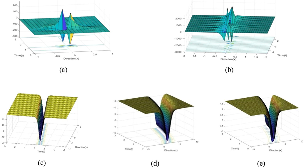
3D plot of the solution of (3.1.12) for the different values.

On the other hand, for the solution function $U_{2} (x, y, t)$ we found anti-bell shape soliton depicted in Fig. 2(a) for the following values of the parameters $α = 1$ , $β = 1$ , $γ = 1$ , $δ = 1$ with in the range $- 5 \leq x \leq 10$ and $0 \leq t \leq 5$ . The nature of the figure of this solution changes for the changes of the parameter $α$ . It depicts singular point-type soliton for $α = - 4, β = 1, γ = 1, δ = 1$ shown in Fig. 2(b).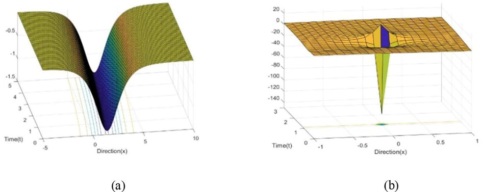

3D plot of the solution of (3.1.13) for the different values.

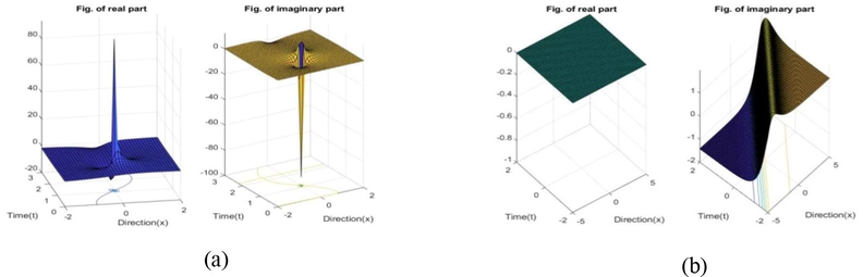
Solution function $U_{3} (x, y, t)$ have both real and imaginary part. We have outlined four different graphs for $U_{3} (x, y, t)$ within the contour $- 2 \leq x, t \leq 2$ . Fig. 3(a) depicts squeezed bell-shape soliton for real part and dark-bright soliton for imaginary part for the values of parameter $α = 1, β = 1, γ = 1, δ = 1.1$ . The solution is highly sensitive in regard to the nonlinear dissipation coefficient $γ$ . In order to clarify, if we change the coefficient $γ$ and choose the values $α = 1, β = 1, γ = - 1, δ = 1.1$ , we found the Fig. 3(b) of the real part that converts into anti-bell type but imaginary part depicts bright-dark soliton. In case of the choice of parameters as $α = - 10, β = - 10, γ = 10, δ = - 10$ , we get anti-lump type soliton and spike type singular periodic wave respectively for real and imaginary part of $U_{3} (x, y, t)$ as shown in Fig. 3(c). In Fig. 3(d) we get nearly similar figure for $U_{3} (x, y, t)$ , with the values $α = - 10, β = - 10, γ = - 10, δ = - 10$ , where real part shows lump type soliton and imaginary part displays spike type singular periodic wave which is also called breather type soliton.

3D plot of the solution of (3.1.14) for the different values.

Since the features of the solution $U_{4} (x, y, t)$ are analogous to the figure of the erstwhile solutions thus these profiles are not depicted to avoid repetition.

4.2

4.2 Figures of the solutions of the KG equation

The acquired stable traveling wave solutions of the KG equation are explained in the figures and estimated the nature of these waves for different values of the parameters using the MATLAB software.

For the first solution function $V_{1} (x, y, t)$ , we obtained smooth kink type figure for the values of the free variables $σ = - 5$ , $μ = 1.1$ and depicted in Fig. 4(a). The nature of $V_{1} (x, y, t)$ varies in rogue wave for the variation of $σ$ and it is illustrated in Fig. 4 (b). The figure is delineated for $σ = 5, μ = 1.1$ with in the interval $- 3 \leq x \leq 3$ and $0 \leq t \leq 5$ .

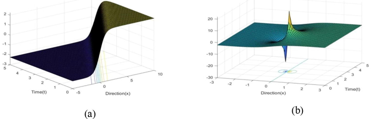
3D plot of the solution of (3.2.10) for the different values.

The other solution $V_{2} (x, y, t)$ supplies anti-bell profile wave revealed in Fig. 5(a) for the parametric values $σ = 1, μ = 1.1$ within the interval $- 5 \leq x \leq 10$ and $0 \leq t \leq 3$ . The same solution represents singular profile if we change the value of $μ$ by $μ = - 1.1$ .

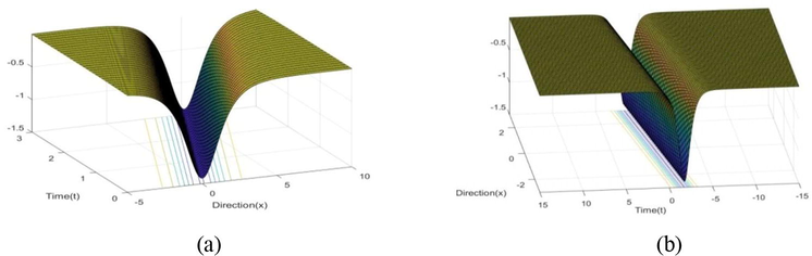
3D plot of the solution of (3.2.11) for the different values.

For $V_{3} (x, y, t)$ we select following values $σ = 2, μ = 1.1$ within the interval $- 2 \leq x \leq 2$ and $0 \leq t \leq 3$ to sketch the graph in Fig. 6(a) which depicts lump and anti-lump wave for real and imaginary part respectively which are both singular point soliton. The solution alters it form for decreasing the free variable $σ$ in Fig. 6(b), and becomes a flat wave for real part and kink type soliton for imaginary part for $σ = 2, μ = 1.1$ .

3D plot of the solution of (3.2.12) for the different values.

It is significant how varieties of solitons are found for various choices of parametric values in a unique manner for the KG equation through this study.

From the results and graph, it is clear that both the equations we discussed in this article provide us diverse solitons, like kink wave, singular point soliton, spiked periodic wave, anti-bell wave, lump type soliton etc. We also acquire some new complex hyperbolic function solutions that have not been submitted to literature beforehand.

5 Comparison of the solutions

We will relate the solutions examined by the sGE method of the generalized Boussinesq equation and the Klein–Gordon equation. In this section, we will also emulate the determined solutions with those ascertained by various researchers of the stated equations using different methods.

5.1

5.1 Comparison of the obtained solutions of the gBE

We establish some general and some new-found solitary wave solutions to the (2 + 1)-dimensional gBE in this research. Nevertheless, this equation have been investigated by the new generalized Jacobi elliptic function method (Huai and Hong, 2004), the Hirota bilinear method (Ma and Deng, 2016), the sine–cosine method (Taşcan and Bekir, 2009), etc. The obtained solutions are compared with those found by Taşcan and Bekir (2009) via the sine–cosine method and presented in Table 1.

Table 1 Comparison of the solutions of the gBE obtained by the sine–cosine method and the sGE method.

Taşcan and Bekir (2009) solutions	Solutions obtained by sGE method
(i) Choose $c = \sqrt{- 4}$ and $u (x, y, t) = U_{2}$ then the solution (3.9) gives	(i) If $α = β = γ = δ = 1$ , then equation (3.1.13) becomes
$U_{2} = - 9 S e c h^{2} (\frac{\sqrt{6}}{2} (x + y - \sqrt{- 4} t)) .$	$U_{2} = 6 S e c h^{2} (x + y - \sqrt{- 4} t) .$

It should be noted that, Taşcan and Bekir (2009) have found three more solution which are not similar with the solutions established in this article. On the other hand, formulating the sGE method, three more different results namely $U_{1}$ , $U_{3}$ and $U_{4}$ of the gBE have achieved that dot not match with the earlier results. Not only that, we have portrayed different shapes of soliton solutions through sGE scheme, such as anti-bell, breather, bright-dark shape soliton etc. which are not found by Taşcan and Bekir (2009).

5.2

5.2 Comparison of the solutions of the KG equation

In the early research, the (2 + 1)-dimensional KG equation has been investigated through the modified simple equation method (Khan and Akbar, 2014) and the modified extended mapping method (Seadawy et al., 2018). These investigations derived the trigonometric and hyperbolic function solutions to the KG equation. In this article, we establish the combination of hyperbolic function solutions for the same equation using the sGE method. Nonetheless, the attained solutions are compared with Khan and Akbar (2014) solutions which are accomplished by the modified simple equation (MSE) method in Table 2:

Table 2 Comparison of the solutions achieved by the MSE method and the SGE method.

Khan and Akbar (2014) solutions	Solutions attained in this article
(i) If $α = σ$ , $β = μ$ and $u_{3, 4} (x, y, t) = V_{1}$ , then the solution (3.19) becomes $V_{1} = \pm \sqrt{\frac{- σ}{μ}} \tanh (\sqrt{\frac{σ}{2 (λ^{2} - 2)}} (x + y - λ t))$ .	(i) Replacing $λ = \frac{1}{2} \sqrt{8 - 2 σ}$ the solution (3.2.10) becomes $V_{1} = \sqrt{\frac{- σ}{μ}} \tanh ((x + y - λ t))$ .
(ii) If $α = σ$ , $β = μ$ and $u_{7, 8} (x, y, t) = V_{1}$ then the solution (3.21) converts $V_{1} = \pm \sqrt{\frac{σ}{μ}} \tan (\sqrt{\frac{σ}{2 (λ^{2} - 2)}} (x + y - λ t))$	(ii) Substituting $λ = \frac{1}{2} \sqrt{8 - 2 σ}$ the solution (3.2.10) becomes $V_{1} = \sqrt{\frac{σ}{μ}} \tan ((x + y - λ t))$ .

Besides, Khan and Akbar (2014) have established two more solutions which are not similar to our solutions. But we have found more two solutions likewise solutions (3.2.11) and (3.2.12) and achieved various type waves like kink, bell and lamb type soliton for the KGE which are not analogous in the earlier investigation. Although, we have discussed the nature of the waves for the stated both equations by changing the values of free parameters.

6 Conclusions

In this article, we extend, analyze the sGE approach and put in use to a couple of higher-dimensional NLEEs, namely the gBE and KG equations. We have attained different types of wave solutions to the formerly stated models, such as breather, rogue, bell-shape, bright-dark, kink and periodic solitons. We identified the nature of the wave profiles and showed that the wave profiles depend on the score of the free parameters. The instance has been analyzed in detail in the results and discussion section. This study demonstrates that the efficacy of the extended sGE method is reliable and an efficient strategy for analyzing higher-dimensional NLEEs and might be impactful to examine higher-dimensional NLEEs in future studies.

Declaration of Competing Interest

The authors declare that they have no known competing financial interests or personal relationships that could have appeared to influence the work reported in this paper.

References

Ablowitz M.J., Segur H., . Solitons and the inverse scattering transform. SIAM, Philadelphia. 1981;127:8043-8055.
[Google Scholar]
Akbar M.A., Ali N.H.M., . Exp-function method for Duffing equation and new solutions of (2+1)-dimensional dispersive long wave equations. Prog. Appl. Math.. 2011;1(2):30-42.
[Google Scholar]
Akbar M.A., Ali N.H.M., . The alternative (G'G)-expansion method and its applications to nonlinear partial differential equations. Int. J. Phys. Sci.. 2011;6(35):7910-7920.
[Google Scholar]
Ali Akbar M., Ali N.H.M., Wang P., . The improved F-expansion method with Riccati equation and its applications in mathematical physics. Cogent Math.. 2017;4(1):1282577.
[CrossRef] [Google Scholar]
Akbar M.A., Ali N.H.M., Hussain J., . Optical soliton solutions to the (2+1)-dimensional Chaffee-Infante equation and the dimensionless form of the Zakharov equation. Adv. Diff. Equa.. 2019;2019:446.
[Google Scholar]
Aksan E.N., Bulut H., Kayhan M., . Some wave simulation properties of the (2+1) dimensional breaking solution equation. ITM (conferences).. 2017;13:01014.
[Google Scholar]
Bai C.-L., Zhao H., . Complex hyperbolic-function method and its applications to nonlinear equations. Phys. Lett. A.. 2006;355(1):32-38.
[Google Scholar]
Baskonus H.M., Bulut H., . Exponential prototype structure for (2+1)-dimensional Boiti-Leon-Pempinelli systems in mathematical physics. Waves Random Complex Media.. 2016;26:189-196.
[Google Scholar]
Deng W., . Finite element method for the space and time fractional Fokker-Planck equation. SIAM J. Numer. Anal.. 2009;47(1):204-226.
[Google Scholar]
Dehghan M., Abbaszadeh M., . A finite difference/finite element technique with error estimate for space fractional tempered diffusion-wave equation. Comput. Math. Appl.. 2018;75(8):2903-2914.
[Google Scholar]
Elwakil S.A., El-labany S.K., Zahran M.A., Sabry R., . Modified extended tanh-function method for solving nonlinear partial differential equations. Phys. Lett A.. 2002;299(2-3):179-188.
[Google Scholar]
Ghanbari B., Gómez-Aguilar J.F., . Optical soliton solutions for the nonlinear Radhakrishnan-Kundu-Lakshmanan equation. Modern Phys. Lett. B.. 2019;33(32):1950402.
[CrossRef] [Google Scholar]
Gu C., Hu H., Zhou Z., eds. Darboux Transformations in Integrable Systems. Dordrecht: Springer Netherlands; 2005.
Gu C., Hu H., . Explicit solutions to the intrinsic generalization for the wave and sine-Gordon equations. Lett. Math. Phys.. 1993;29(1):1-11.
[Google Scholar]
He J., . Variational iteration method for delay differential equations. Commun. Nonlin. Sci. Numer. Simulat.. 1997;2(4):235-236.
[Google Scholar]
Hosseini K., Aligoli M., Mirzazadeh M., Eslami M., Gómez-Aguilar J.F., . Dynamics of rational solutions in a new generalized Kadomtsev-Petviashvili equation. Modern Phys. Lett. B.. 2019;33(35):1950437.
[CrossRef] [Google Scholar]
Huai-Tang C., Hong-Qing Z., . New double periodic and multiple soliton solutions of the generalized (2+1) dimensional Boussinesq equation. Chaos Soliton Fractal.. 2004;20(4):765-769.
[Google Scholar]
Iftikhar, A., Ghafoor, A., Zubair, T., Firdous, S., Mohyud-Din S.T., -expansion method for traveling wave solutions of (2+1)-dimensional generalized KdV, Sine-Gordon and Landau-Ginzburg-Higgs equations. Scientific Res. Essays. 8(28), 1349-1359.
Inc M., . The approximate and exact solutions of the space- and time-fractional Burgers equations with initial conditions by variational iteration method. J. Math. Anal. Appl.. 2008;345(1):476-484.
[Google Scholar]
Islam M.E., Barman H.K., Akbar M.A., . Search for interactions of phenomena described by the coupled Higgs field equation through analytical solutions. Opt. Quant. Elect.. 2020;52:468.
[Google Scholar]
Khan, K., Akbar, M.A., 2013. Exact and solitary wave solutions for the Tzitzeica-Dodd-Bullough and the modified KdV-Zakharov-Kuznetsov equations using the modified simple equation method. Ain Shams Engg. J. 4(4), 903-909.
Khan, K. Akbar, M.A., Exact solutions of the (2+1)-dimensional cubic Klein-Gordon equation and the (3+1)-dimensional Zakharov-Kuznetsov equation using the modified simple equation method. J. Assoc. Arab Univ. Basic Appl. Sci. 15, 74-81.
Khater M.M.A., . Exact traveling wave solutions for an important mathematical physics model. J. Appl. Math. Bioinfor.. 2016;6:37-48.
[Google Scholar]
Korkmaz A., Hepson O.E., Hosseini K., Rezazadeh H., Eslami M., . Sine-Gordon expansion method for exact solutions to conformable time fractional equations in RLW-class. J. King Saud Univ.-Sci.. 2020;32(1):567-574.
[Google Scholar]
Ma H.-C., Deng A.-P., . Lump solution of (2+1)-dimensional Boussinesq equation. Commun. Theor. Phys.. 2016;65(5):546-552.
[Google Scholar]
Morales-Delgado V.F., Gómez-Aguilar J.F., Baleanu D., . A new approach to exact optical soliton solutions for the nonlinear Schrödinger equation. Eur. Phys. J. Plus.. 2018;133(5):189.
[Google Scholar]
Nuruddeen R.I., Nass A.M., . Exact solitary wave solution for the fractional and classical GEW-Burgers equations: an application of Kudryashov method. J. Taibah Univ. Sci.. 2018;12(3):309-314.
[Google Scholar]
Osman M.S., Ali K.K., Gómez-Aguilar J.F., . A variety of new optical soliton solutions related to the nonlinear Schrödinger equation with time-dependent coefficients. Optik.. 2020;222:165389.
[CrossRef] [Google Scholar]
Saha Ray S., . A new analytical modelling for nonlocal generalized Riesz fractional sine-Gordon equation. J. King Saud Univ.-Sci.. 2016;28(1):48-54.
[Google Scholar]
Seadawy A.R., Lu D.-C., Arshad M., . Stability analysis of solitary wave solutions for coupled and (2+1)-dimensional cubic Klein-Gordon equations and their applications. Commun. Theor. Phys.. 2018;69(6):676.
[CrossRef] [Google Scholar]
Sedeeg A.K.H., Nuruddeen R.I., Gómez-Aguilar J.F., . Generalized optical soliton solutions to the (3+ 1)-dimensional resonant nonlinear Schrödinger equation with Kerr and parabolic law nonlinearities. Opt. Quant. Elect.. 2019;51(6):173.
[Google Scholar]
Shi Y.R., Xu X.J., Wu Z.X., . Application of the homotopy analysis method to solving nonlinear evolution equations. Acta Physica Sinica.. 2006;55(4):1555-1560.
[Google Scholar]
Taşcan F., Bekir A., . Analytic solutions of the (2+1)-dimensional nonlinear evolution equations using the sine-cosine method. Appl. Math. Comput.. 2009;215(8):3134-3139.
[Google Scholar]
Triki H., Yildirim A., Hayat T., Aldossary O.M., Biswas A., . Shock wave solution of the Benney-Luke equation. Rom. J Phys.. 2012;57:1029-1034.
[Google Scholar]
Wang M., Li X., Zhang J., . The (G'G)-expansion method and travelling wave solutions of nonlinear evolution equations in mathematical physics. Phys. Lett. A. 2008;372:417-423.
[Google Scholar]
Wang G., Yang K., Gu H., Guan F., Kara A.H., . A (2+1)-dimensional sine-Gordon and sinh-Gordon equations with symmetries and kink wave solutions. Nuclear Phys. B.. 2020;953:114956.
[CrossRef] [Google Scholar]
Wazwaz, A.M., Sine-Cosine method for handling nonlinear wave equations. Math. Comput. Model. 40, 499-508.
Xie J., Zhang Z., Liang D., . A conservative splitting difference scheme for the fractional-in-space Boussinesq equation. Appl. Numer. Math.. 2019;143:61-74.
[Google Scholar]
Yépez-Martínez H., Gómez-Aguilar J.F., Baleanu D., . Beta-derivative and sub-equation method applied to the optical solitons in medium with parabolic law nonlinearity and higher order dispersion. Optik.. 2018;155:357-365.
[Google Scholar]

Introduction

Methodology

Extraction of solution using the extended sGE approach

The generalized Boussinesq equation
The KG equation

Results and discussion and graphical representations

Figures of the solutions of the gBE
Figures of the solutions of the KG equation

Comparison of the solutions

Comparison of the obtained solutions of the gBE
Comparison of the solutions of the KG equation

Conclusions

Fulltext Views
28

PDF downloads
24

View/Download PDF
Download Citations

BibTeX
RIS

Show Sections

[1] Ablowitz M.J., Segur H., . Solitons and the inverse scattering transform. SIAM, Philadelphia. 1981;127:8043-8055.
[Google Scholar]

[2] Akbar M.A., Ali N.H.M., . Exp-function method for Duffing equation and new solutions of (2+1)-dimensional dispersive long wave equations. Prog. Appl. Math.. 2011;1(2):30-42.
[Google Scholar]

[3] Akbar M.A., Ali N.H.M., . The alternative (G'G)-expansion method and its applications to nonlinear partial differential equations. Int. J. Phys. Sci.. 2011;6(35):7910-7920.
[Google Scholar]

[4] Ali Akbar M., Ali N.H.M., Wang P., . The improved F-expansion method with Riccati equation and its applications in mathematical physics. Cogent Math.. 2017;4(1):1282577.
[CrossRef] [Google Scholar]

[5] Akbar M.A., Ali N.H.M., Hussain J., . Optical soliton solutions to the (2+1)-dimensional Chaffee-Infante equation and the dimensionless form of the Zakharov equation. Adv. Diff. Equa.. 2019;2019:446.
[Google Scholar]

[6] Aksan E.N., Bulut H., Kayhan M., . Some wave simulation properties of the (2+1) dimensional breaking solution equation. ITM (conferences).. 2017;13:01014.
[Google Scholar]

[7] Bai C.-L., Zhao H., . Complex hyperbolic-function method and its applications to nonlinear equations. Phys. Lett. A.. 2006;355(1):32-38.
[Google Scholar]

[8] Baskonus H.M., Bulut H., . Exponential prototype structure for (2+1)-dimensional Boiti-Leon-Pempinelli systems in mathematical physics. Waves Random Complex Media.. 2016;26:189-196.
[Google Scholar]

[9] Deng W., . Finite element method for the space and time fractional Fokker-Planck equation. SIAM J. Numer. Anal.. 2009;47(1):204-226.
[Google Scholar]

[10] Dehghan M., Abbaszadeh M., . A finite difference/finite element technique with error estimate for space fractional tempered diffusion-wave equation. Comput. Math. Appl.. 2018;75(8):2903-2914.
[Google Scholar]

[11] Elwakil S.A., El-labany S.K., Zahran M.A., Sabry R., . Modified extended tanh-function method for solving nonlinear partial differential equations. Phys. Lett A.. 2002;299(2-3):179-188.
[Google Scholar]

[12] Ghanbari B., Gómez-Aguilar J.F., . Optical soliton solutions for the nonlinear Radhakrishnan-Kundu-Lakshmanan equation. Modern Phys. Lett. B.. 2019;33(32):1950402.
[CrossRef] [Google Scholar]

[13] Gu C., Hu H., Zhou Z., eds. Darboux Transformations in Integrable Systems. Dordrecht: Springer Netherlands; 2005.

[14] Gu C., Hu H., . Explicit solutions to the intrinsic generalization for the wave and sine-Gordon equations. Lett. Math. Phys.. 1993;29(1):1-11.
[Google Scholar]

[15] He J., . Variational iteration method for delay differential equations. Commun. Nonlin. Sci. Numer. Simulat.. 1997;2(4):235-236.
[Google Scholar]

[16] Hosseini K., Aligoli M., Mirzazadeh M., Eslami M., Gómez-Aguilar J.F., . Dynamics of rational solutions in a new generalized Kadomtsev-Petviashvili equation. Modern Phys. Lett. B.. 2019;33(35):1950437.
[CrossRef] [Google Scholar]

[17] Huai-Tang C., Hong-Qing Z., . New double periodic and multiple soliton solutions of the generalized (2+1) dimensional Boussinesq equation. Chaos Soliton Fractal.. 2004;20(4):765-769.
[Google Scholar]

[18] Iftikhar, A., Ghafoor, A., Zubair, T., Firdous, S., Mohyud-Din S.T., -expansion method for traveling wave solutions of (2+1)-dimensional generalized KdV, Sine-Gordon and Landau-Ginzburg-Higgs equations. Scientific Res. Essays. 8(28), 1349-1359.

[19] Inc M., . The approximate and exact solutions of the space- and time-fractional Burgers equations with initial conditions by variational iteration method. J. Math. Anal. Appl.. 2008;345(1):476-484.
[Google Scholar]

[20] Islam M.E., Barman H.K., Akbar M.A., . Search for interactions of phenomena described by the coupled Higgs field equation through analytical solutions. Opt. Quant. Elect.. 2020;52:468.
[Google Scholar]

[21] Khan, K., Akbar, M.A., 2013. Exact and solitary wave solutions for the Tzitzeica-Dodd-Bullough and the modified KdV-Zakharov-Kuznetsov equations using the modified simple equation method. Ain Shams Engg. J. 4(4), 903-909.

[22] Khan, K. Akbar, M.A., Exact solutions of the (2+1)-dimensional cubic Klein-Gordon equation and the (3+1)-dimensional Zakharov-Kuznetsov equation using the modified simple equation method. J. Assoc. Arab Univ. Basic Appl. Sci. 15, 74-81.

[23] Khater M.M.A., . Exact traveling wave solutions for an important mathematical physics model. J. Appl. Math. Bioinfor.. 2016;6:37-48.
[Google Scholar]

[24] Korkmaz A., Hepson O.E., Hosseini K., Rezazadeh H., Eslami M., . Sine-Gordon expansion method for exact solutions to conformable time fractional equations in RLW-class. J. King Saud Univ.-Sci.. 2020;32(1):567-574.
[Google Scholar]

[25] Ma H.-C., Deng A.-P., . Lump solution of (2+1)-dimensional Boussinesq equation. Commun. Theor. Phys.. 2016;65(5):546-552.
[Google Scholar]

[26] Morales-Delgado V.F., Gómez-Aguilar J.F., Baleanu D., . A new approach to exact optical soliton solutions for the nonlinear Schrödinger equation. Eur. Phys. J. Plus.. 2018;133(5):189.
[Google Scholar]

[27] Nuruddeen R.I., Nass A.M., . Exact solitary wave solution for the fractional and classical GEW-Burgers equations: an application of Kudryashov method. J. Taibah Univ. Sci.. 2018;12(3):309-314.
[Google Scholar]

[28] Osman M.S., Ali K.K., Gómez-Aguilar J.F., . A variety of new optical soliton solutions related to the nonlinear Schrödinger equation with time-dependent coefficients. Optik.. 2020;222:165389.
[CrossRef] [Google Scholar]

[29] Saha Ray S., . A new analytical modelling for nonlocal generalized Riesz fractional sine-Gordon equation. J. King Saud Univ.-Sci.. 2016;28(1):48-54.
[Google Scholar]

[30] Seadawy A.R., Lu D.-C., Arshad M., . Stability analysis of solitary wave solutions for coupled and (2+1)-dimensional cubic Klein-Gordon equations and their applications. Commun. Theor. Phys.. 2018;69(6):676.
[CrossRef] [Google Scholar]

[31] Sedeeg A.K.H., Nuruddeen R.I., Gómez-Aguilar J.F., . Generalized optical soliton solutions to the (3+ 1)-dimensional resonant nonlinear Schrödinger equation with Kerr and parabolic law nonlinearities. Opt. Quant. Elect.. 2019;51(6):173.
[Google Scholar]

[32] Shi Y.R., Xu X.J., Wu Z.X., . Application of the homotopy analysis method to solving nonlinear evolution equations. Acta Physica Sinica.. 2006;55(4):1555-1560.
[Google Scholar]

[33] Taşcan F., Bekir A., . Analytic solutions of the (2+1)-dimensional nonlinear evolution equations using the sine-cosine method. Appl. Math. Comput.. 2009;215(8):3134-3139.
[Google Scholar]

[34] Triki H., Yildirim A., Hayat T., Aldossary O.M., Biswas A., . Shock wave solution of the Benney-Luke equation. Rom. J Phys.. 2012;57:1029-1034.
[Google Scholar]

[35] Wang M., Li X., Zhang J., . The (G'G)-expansion method and travelling wave solutions of nonlinear evolution equations in mathematical physics. Phys. Lett. A. 2008;372:417-423.
[Google Scholar]

[36] Wang G., Yang K., Gu H., Guan F., Kara A.H., . A (2+1)-dimensional sine-Gordon and sinh-Gordon equations with symmetries and kink wave solutions. Nuclear Phys. B.. 2020;953:114956.
[CrossRef] [Google Scholar]

[37] Wazwaz, A.M., Sine-Cosine method for handling nonlinear wave equations. Math. Comput. Model. 40, 499-508.

[38] Xie J., Zhang Z., Liang D., . A conservative splitting difference scheme for the fractional-in-space Boussinesq equation. Appl. Numer. Math.. 2019;143:61-74.
[Google Scholar]

[39] Yépez-Martínez H., Gómez-Aguilar J.F., Baleanu D., . Beta-derivative and sub-equation method applied to the optical solitons in medium with parabolic law nonlinearity and higher order dispersion. Optik.. 2018;155:357-365.
[Google Scholar]

Extension of the sine-Gordon expansion scheme and parametric effect analysis for higher-dimensional nonlinear evolution equations

Abstract

Keywords

sGEM

gBE

KGE

Soliton solutions

1 Introduction

2 Methodology

3 Extraction of solution using the extended sGE approach

3.1 The generalized Boussinesq equation

3.2 The KG equation

4 Results and discussion and graphical representations

4.1 Figures of the solutions of the gBE

4.2 Figures of the solutions of the KG equation

5 Comparison of the solutions

5.1 Comparison of the obtained solutions of the gBE

5.2 Comparison of the solutions of the KG equation

6 Conclusions

Declaration of Competing Interest

References

Suggested read for related articles: