

Translate this page into:
Explicit finite difference analysis of an unsteady MHD flow of a chemically reacting Casson fluid past a stretching sheet with Brownian motion and thermophoresis effects
⁎Corresponding authors. mohammad.shakhaoath.khan@rmit.edu.au (Md. Shakhaoath Khan), sfahmmed@yahoo.com (Sarder Firoz Ahmmed)
-
Received: ,
Accepted: ,
This article was originally published by Elsevier and was migrated to Scientific Scholar after the change of Publisher.
Peer review under responsibility of King Saud University.
Abstract
This study intends to elaborate the heat and mass transfer analysis of Casson nanofluid flow past a stretching sheet together with magnetohydrodynamics (MHD), thermal radiation and chemical reaction effects. The boundary layer approximations established the governing equations, i.e., time-subservient momentum, energy and diffusion balance equations. An explicit finite difference scheme was implemented as a numerical technique where Compaq Visual Fortran 6.6.a programming code is also developed for simulating the fluid flow system. In order to accurateness of the numerical technique, a stability and convergence analysis was carried out where the system was found converged at Prandtl number, Pr ≥ 0.062 and Lewis number, Le ≥ 0.025 when τ = 0.0005, ΔX = 0.8 and ΔY = 0.2. The non-dimensional outcomes are apprehended here which rely on various physical parameters. The impression of these various physical parameters on momentum and thermal boundary layers along with concentration profiles are discussed and displayed graphically. In addition, the impact of system parameters on Cf, Nu and Sh profiles with streamlines and isothermal lines are also discussed.
Keywords
Casson nanofluid
Heat and mass transfer
MHD
Thermal radiation
Stretching sheet

Nomenclature
- B0
-
magnetic component, [Wbm−2]
- C
-
Dimensionless concentration, [–]
- Cf
-
skin friction coefficient, [–]
- cp
-
specific heat, [Jkg−1K−1]
-
concentration at wall surface
-
nanoparticle concentration away from surface
- DT
-
thermophoresis diffusion coefficient
- DB
-
Brownian diffusion coefficient
- Ec
-
Eckert number, [–]
- g
-
gravitational acceleration, [ ]
- Kr
-
chemical reaction parameter, [–]
- k*
-
mean absorption coefficient, [–]
- Le
-
Lewis number, [–]
- M
-
magnetic parameter, [–]
- N
-
stretching/shrinking parameter, [–]
- Nt
-
thermophoresis parameter, [–]
- Nb
-
Brownian parameter, [–]
- Nu
-
Nusselt number, [–]
- Pr
-
Prandtl number, [–]
- qr
-
radiative heat flux, [kgm−2]
- Q
-
heat generation parameter, [–]
- Ra
-
radiation parameter, [–]
- Sh
-
mass transfer coefficient (Sherwood number), [–]
- t
-
dimensional time, [s]
- T
-
fluid temperature, [K]
-
temperature away from the surface
-
velocity component in x, y-direction, [ms−1]
- x, y
-
cartesian coordinate system
- β
-
Casson fluid parameter
- υ
-
kinematic viscosity, [m2s−1]
- τ
-
dimensionless time, [–]
- ρ
-
fluid density, [kg m−3]
- κ
-
thermal conductivity, [Wm−1 K−1]
- σ
-
Stefan-Boltzmann constant, [Wm− K−4]
Greek symbols
1 Introduction
In the past decade, advance in nanotechnology has initiated a lot of expectation for the experts in industries, engineering and technologies field. Nanofluids are one of the wonder of such evolution. This type of fluids is basically originated from the intermixing of base fluid and nanometer-sized particles; however, nanoparticles usually have supreme thermal conductivity compared to their base fluids. Nanofluids have a comprehensive range of applications in biomedical, cancer therapeutics, solar industry, defence sector etc. Akbar et al. (2012) introduced peristaltic flow in nanofluids in a diverging tube and found that temperature profiles of the fluid phase increase for developing data of Brownian and thermophoretic parameters while the opposite behaviour observed in the concentration profile. By incorporating the application of HAM-based Mathematica package BVPh 2.0, Farooq et al. (2015) also exhibited the attitude of the above mentioned parameters in a hydromagnetic Falkner–Skan nanofluid flow. Analysis of heat transfer together with viscous dissipation and Joule heating properties in a stagnation-point flow of viscous radiative nanofluid for solar energy was investigated by Mushtaq et al. (2014). Sheikholeslami et al. (2017a, 2017b) discussed heat transfer flow of forced convective nanofluid with the influence of external magnetic source using both Lattice Boltzmann Method (LBM) and control-based volume finite element method (CVFEM).
Numerous researchers and scientists were fascinated by the characteristics of non-Newtonian fluid namely Casson fluid and stretching sheet because of their extensive applications in many industries. Casson fluid is a shear thinning liquid in which at zero shear rates it will have infinite viscosity and vice-versa. Hayat et al. (2012) observed the behaviour of Casson fluid which was flowing on a stretched surface with a convective boundary condition structure. Imtiaz et al. (2016) extended Hayat et al. (2012)’s study by incorporating nanoparticles and they did their experiment on stretching cylinder. Khan et al. (2017a) explored MHD Casson fluid stagnation point flow together with the reaction of homogeneous-heterogeneous properties. Tamoor et al. (2017) examined Newtonian heating characteristics of MHD Casson fluid flow initiated by a stretched cylinder moving with linear velocity. Zaigham Zia et al. (2018) premeditated Soret-Dufour effects on Casson fluid, which was flowing on exponentially heated surface with space-dependent heat source.
The impression of thermal radiation on the fluid flow is noteworthy to analyse as many engineering and industrial applications can be comprehended for example reactor safety, geothermal systems, heat internment etc. Hayat et al. (2015) carried out the impact of non-linear thermal radiation on viscous nanofluid flow resulting from stretched surface. Further studies due to the nonlinear thermal radiation impacts on stagnation point flow of nanofluid towards a stretched surface was apprehended by Hayat et al. (2016a). Recently several researchers (Hayat et al., 2018a, 2018b; Khan et al., 2017b, 2017c) are involved in this area to improve the heat and mass transfer in nanotechnology.
By making use of the above studies, the intention of the current investigation is to pursue the thermophoretic and Brownian motion parameters impact on unsteady hydromagnetic chemically reactive Casson nanofluid flow because of stretching on a plane surface. The present study is concerned with modified Darcy’s law where for detail description, the reader can refer to the recent literature (Hayat et al., 2017, 2016b; Husain et al., 2008; Tanveer et al., 2017). EFDM analysis together with a convergence and stability experiment (Arifuzzaman et al., 2017; Arifuzzaman et al., 2018; Khan et al., 2016, 2012) have been done. The impressions of relevant parameters are being exhibited graphically on velocity, concentric and temperature fields. However, the fields of Cf, Nu and Sh with streamlines and isothermal lines are also displayed with graphical and tabular representation. Furthermore, for the validation of the present study, qualitative comparisons with previous literature are also shown.
2 Mathematical analysis
Under thermal radiation impact, an unsteady higher order chemically reactive two-dimensional laminar Casson nanofluid flow resulting from a stretched surface has been considered. A transverse magnetic field (B0 = By) is also exerted here.
represents the velocity on a stretched surface and the upward direction depicts the x-axis whilst y-axis is considered normal to the surface (Fig. 1). Let, y ≥ 0 exhibits the flow direction. The species concentration and plate temperature increased at t > 0. Here
and
are surface temperature and concentration whereas the concentration and temperature away from the plate are
and
.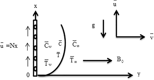
Physical configuration.
The rheological equation of Casson fluid flow (Mukhopadhyay et al., 2013) has been considered as follows:
Under these considerations the dimensional fundamental equations can be expressed for this sort of flow as (Naramgari and Sulochana, 2016; Raju et al., 2016):
Therefore Eq. (4) becomes,
Representing dimensionless quantities as,
Thus, the dimensionless equations are achieved as,
Also, the corresponding boundary conditions are
The following expressions present the physical quantities, skin friction coefficient, Sherwood number and Nusselt number,
The stream function ψ satisfies continuity equation and the velocity components associate as, .
3 Numerical computation
For solving Eqs. (9)–(13), an explicit finite difference scheme has been carried out. Because of that a flow field of rectangular region is taken. This territory is partitioned into grid lines and is collateral to X and Y axes.
Here, X and Y axis are perpendicular and in normal direction respectively (Fig. 2). Here, the height of the plate Xmax (=100) and Ymax (=25) are taken as
. Toward X and Y axes the grid spacing number are m = 125 and n = 125. The constant mesh sizes are considered as
and
towards x and y-axes with smaller time step
. Now,
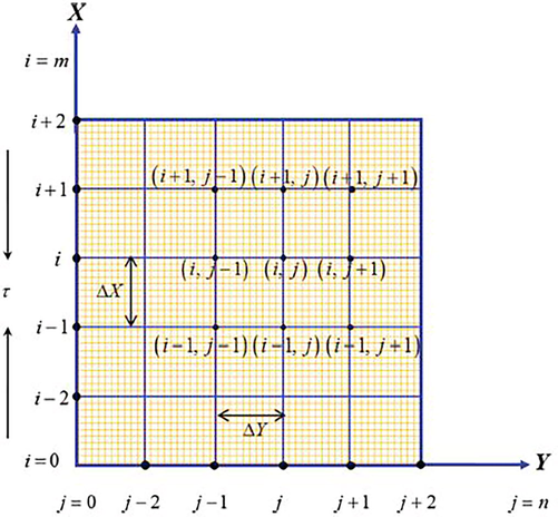
Finite difference grid spacing.
The associated boundary conditions become,
4 Stability and convergence test
It is significant to carry out the stability analysis as well as convergence test of the given problem as finite difference scheme is being implemented explicitly. The probable stability criteria of the scheme for constant mesh sizes are introduced as follows. Because, Δτ does not evident in Eq. (15), it will be overpassed. At an arbitrary time τ = 0, for U, T and C the general terms of Fourier expansion are all
. Here,
. At time τ, the following equations can be obtained:
Therefore, .
For different values of T′ the study is difficult. A small-time step Δτ → 0 is considered. Thus,
in accordance to previous consideration the following expression can be obtained:
Thus, Eigenvalues of T′ are achieved as λ1 = A1, λ2 = A2 and λ3 = A4. These Eigenvalues should not surpass unity in modulus. Therefore, the following stability postulate as
. Choosing,
are obtained.Here a′, b′, c′ and d′ all are real and positive number. Considering, U = ‘+’ and V = ‘−’. So, the maximum modulus of A1, A2 and A4 occurs when
, where n = m = odd integers. Therefore,
The most negative considerable values of A1, A2 and A4 are −1. Hence the stability conditions are:
The primary boundary criterions are . The convergence criterion for the current problem would be established for when Δτ = 0.0005, ΔX = 0.8 and ΔY = 0.2.
5 Results and discussion
The outcomes of the work have been attained by imposing the finite difference system explicitly. The conjectural solutions have been achieved for different parameters for recapitulating the outcomes. To examine the physical status of the problem, the non-dimensional momentum, thermal, fluid concentration, heat transfer coefficient, skin friction coefficient, mass transfer coefficient along with streamlines and isothermal lines has been experimented numerically for stretching surface corresponding to the given boundary conditions. The present numerical simulation was qualitatively validated with the studies of Khan et al. (2012) and Falana et al. (2016) where the values of default parameters M = 2.0, 4.0, Ec = 0.01, Q = 1.0, β = 0.2, 8.0, 10.0, Kr = 1.5, p = 2.0, Kp = 0.01, 1.0, Le = 5, 10, Pr = 1.0 (air), Ra = 1.5, 2.0, Nt = 0.5, N = 1.0, −1.0 and Nb = 0.3 were chosen (see Table 1).
Increased Parameter
Present Result
Khan et al. (2012)
Falana et al. (2016)
U
T
U
T
U
T
M
Dec
Dec
N
Inc
Inc
Pr
Dec
Dec
Nb
Inc
Inc
Inc
Nt
Inc
Inc
In addition to the numerical accuracy, the influence of present physical parameters on skin friction profiles are compared with those of Naramgari and Sulochana (2016) and a good agreement is observed (see Table 2) wherein both analysis, Cf declines as M and Kp increase and interestingly Ra shows no indicatory change on Cf.
Parameter
Naramgari and Sulochana (2016)
Parameter
Present result
M
Ra
Kp
Cf
M
Ra
Kp
Cf
1
1
0.5
−1.851350
2
2
1
−1.83712
2
1
0.5
−2.137573
4
2
1
−1.85808
3
1
0.5
−2.386029
6
2
1
−1.87884
1
1
0.5
−1.851350
2
2
1
−1.83712
1
2
0.5
−1.851350
2
3
1
−1.83712
1
3
0.5
−1.851350
2
4
1
−1.83712
1
1
0.5
−1.851350
2
2
1
−1.83712
1
1
1.0
−2.000248
2
2
1.5
−1.86849
1
1
1.5
−2.137573
2
2
2.5
−1.92982
Figs. 3–18 display the graphical illustration of the given problem. Moreover, a tabular analysis has been presented to exhibit the effects of Nt and Nb on Nu and Sh profiles. In addition, for the case of shrinking the influence of β on momentum boundary layer is also discussed by a tabular analysis.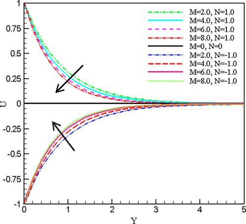
The impression of M on U.
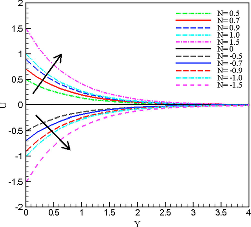
The impression of N on U.
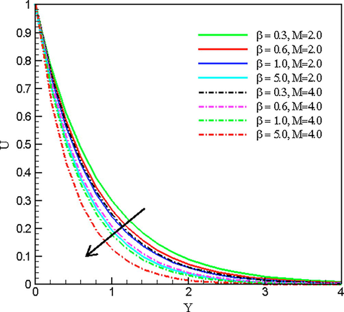
The impression of β on U.
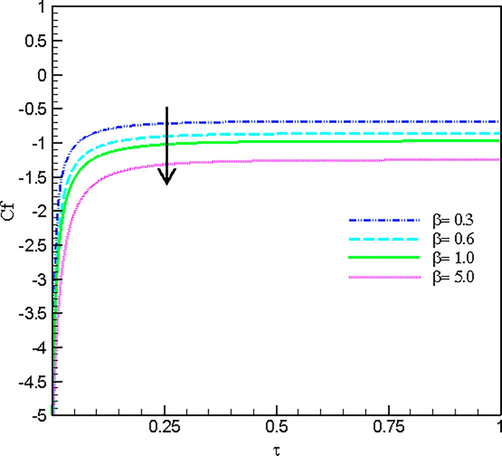
The impression of β on Cf.
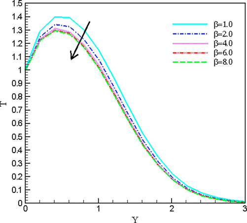
The impression of β on T.
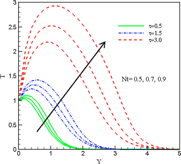
The impression of Nt on T.
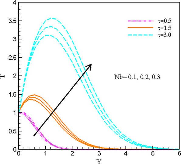
The impression of Nb on T.
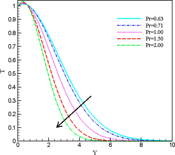
The impression of Pr on T.
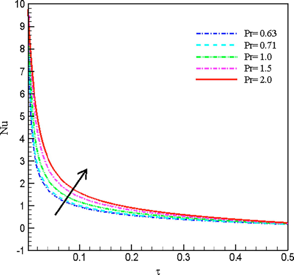
The impression of Pr on Nu.
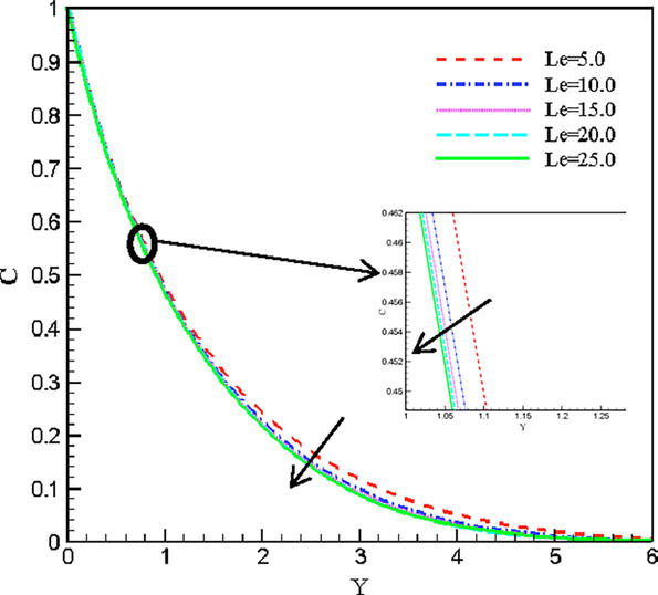
The impression of Le on C.
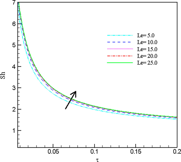
The impression of Le on Sh.
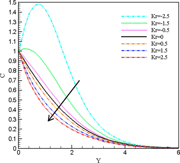
The impression of Kr on C.
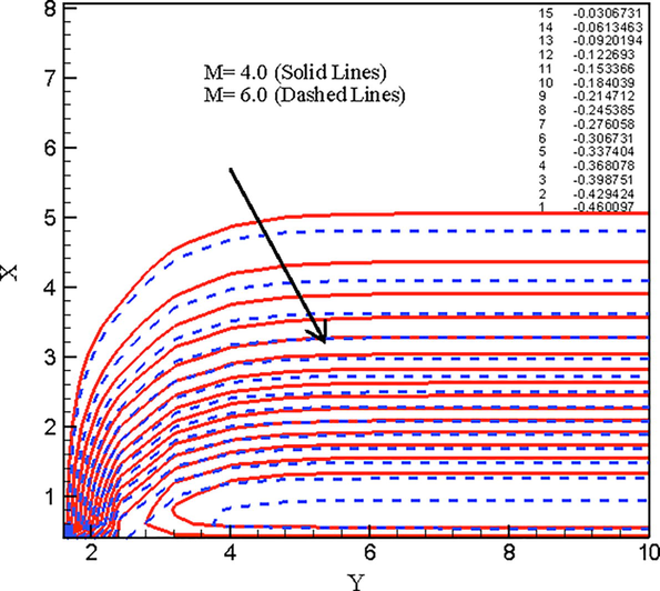
Streamlines for M = 4.0, 6.0.
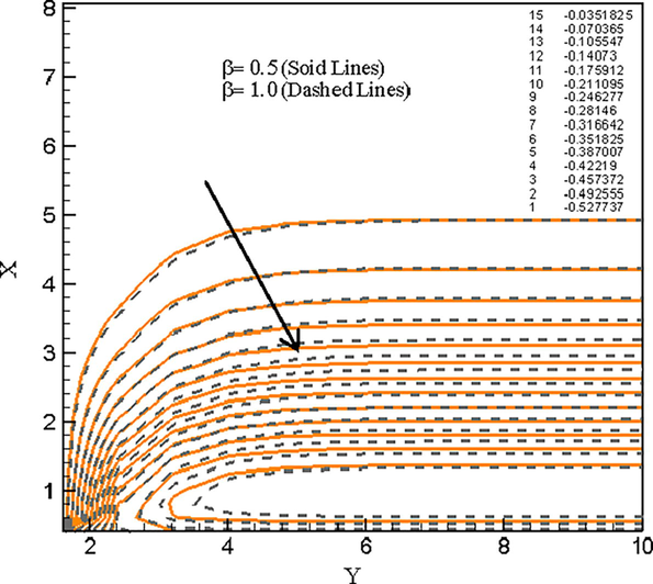
Streamlines for β = 0.5,1.0.
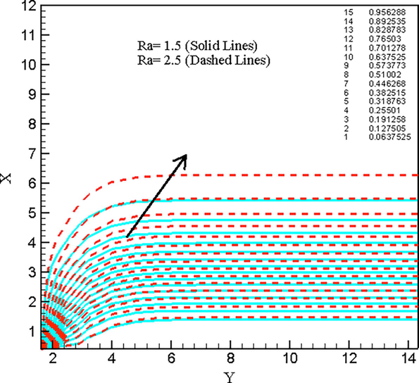
Isothermal lines for Ra = 1.5, 2.5.
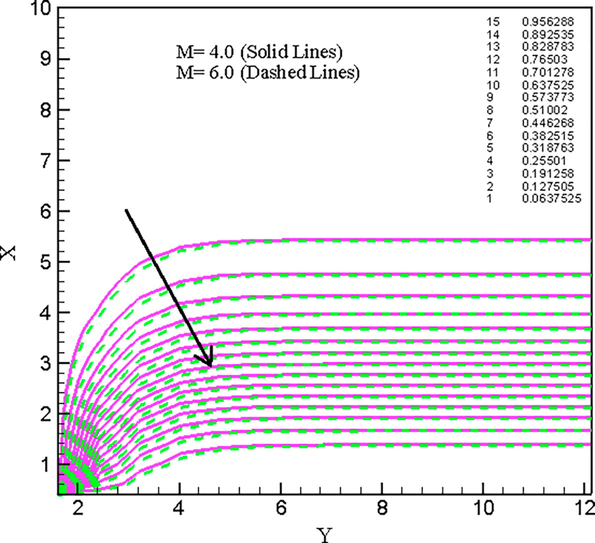
Isothermal lines for M = 4.0, 6.0.
Fig. 3 demonstrates the influence of magnetic parameter, M, upon momentum boundary layers, U, for shrinking (N = −1.0) and stretching (N = 1.0). Generally, the large-scale data of M generates a resistive force called Lorentz force that suppresses the fluid motion. It is undeniable from graph that the momentum boundary layers are diminishing for stretching (N = 1.0) and the Lorentz force enhance the velocity profiles for shrinking (N = −1.0). The influence of stretching and shrinking parameters on momentum boundary layers are experimented in Fig. 4. Herein for increasing stretching parameters the velocity profiles are developing and opposite phenomena is observed for shrinking. Physically, if the values of Casson parameter enhance then the yield stress reduces, and it inhibits the fluid velocity such that it creates a competing force in the fluid flow. Figs. 5–7 display Casson parameter (β) dominance on momentum boundary layers, skin friction coefficient and thermal boundary layers. It is viewed from Fig. 5, the velocity profiles decrease for the increment of Casson parameter when M = 2.0, 4.0 respectively.
In this observation (M = 2.0), the velocity profiles decrease 3.21%, 2.34% and 4.86% for β = 0.3 to 0.6, β = 0.6 to 1.0 and β = 1.0 to 5.0 respectively. A similar act occurred for M = 4.0. It is interesting to observe that, for M = 4.0, Casson parameter is retarding the fluid flow mostly. As it is mentioned earlier, when magnetic field intensity develops then Lorentz force suppress the flow significantly. Here the above incident reflects that when both Casson and magnetic parameters are developing, the velocity fields are declining more rapidly. However, an interesting phenomenon is observed for shrinking. Here, velocity profiles are boosting (Table 3) as the Casson parameter rises.
β
U
0.3
−0.24774
0.6
−0.20447
1.0
−0.17594
5.0
−0.12433
In addition, Skin friction and temperature profiles (Figs. 6 and 7) represent the similar behaviour that happened on velocity profiles for different Casson parameters. Because, when Casson parameter is declining the velocity fields then the fluid particle wouldn’t collide significantly as a result temperature profiles go down. In order to explain the impressions of thermophoretic and Brownian parameters on temperature fields, Figs. 8 and 9 is exhibited at different non-dimensional time τ = 0.5, 1.5, 3.0. At different time steps the thermal boundary layer increases as both thermophoretic (Nt ≥ 0.5), as well as Brownian motion parameters (Nb ≥ 0.1), increases because fluid temperature gets raise due to the uncontrolled motion of nanoparticles.
From Figs. 10 and 11, the influence of Prandtl number, Pr, upon temperature and heat transfer coefficient profiles for Casson fluid can be noticed. Fig. 10 depicts due to increment in Pr; temperature profiles rise near the wall at Y = 0.20161. Furthermore, it declines away from the wall at Y = 0.80645 (after the intersecting point) such that it decreases with increasing Pr and reverse incident is noticed in heat transfer coefficient profiles (Fig. 11). Here the curve increases 25.22%, 62.28%, 55.98% and 29.84% as Prandtl number changes from 0.63 to 0.71, 0.71 to 1.0, 1.0 to 1.5 and 1.5 to 2.0. Figs. 12 and 13 clarify the variations of nanoparticle concentration and Sh profiles for diversified data of Lewis number, Le.
Here for increasing values of Le the concentric profiles decrease but interestingly the mass transfer coefficient profiles increase. For Casson fluid, the dominance of chemical reaction Kr, parameters on concentric profile is shown in Fig. 14. It is perceived that, chemical reaction for the destructive case (Kr = 0.5, 1.5, 2.5) were obstructing the concentric boundary layers more effectively rather than constructive case (Kr = −0.5, −1.5, −2.5). Thus, for both cases the boundary layers are declining. So, it can be concluded that destructive chemical reactions are declining the Casson fluid concentration effectively rather than constructive reactions. From Table 4, it can be observed that, for the increment in Nt and Nb, Nusselt number, Nu, diminishes. Whereas Sherwood number, Sh, diminishes as Nt progresses and a reverse situation is observed for Nb.
Nt
Nb
Nu
Sh
0.50
0.30
4.98988
5.12868
0.70
0.30
4.96606
4.79784
0.90
0.30
4.94197
4.46925
0.50
0.30
4.98988
5.12868
0.50
0.50
4.97134
5.46444
0.50
0.70
4.95271
5.60838
The advanced visualisation of fluid profiles can be exhibited by using streamlines and isothermal lines. Line views from Figs can observe these phenomena. 15 to 18 with contour legend. Here, Figs. 15 and 16 explain the impression of magnetic parameter and Casson parameter on streamlines. However, the isothermal lines are exhibited to explain the impact of radiation and magnetic parameters (Figs. 17 and 18). We can see that, in Figs. 15 and 16 the magnetic and Casson parameters are acting as retarding parameters and decelerating the fluid motion as M and β develops from 4.0 to 6.0 and 0.5 to 1.0 respectively within the boundary region. On the other hand, Fig. 17 illustrates that the energy of fluids develops rapidly and molecules get heated up for strong radiation parameters (Ra = 1.5, 2.5) which render increment to thermal boundary layer thickness. A complete opposite phenomenon is experienced in Fig. 18 for large magnetic parameter (M = 4.0, 6.0).
6 Conclusions
The specific findings of this study are summarised below:
-
Due to rising in M, Kp, N (=−1.0) and β respectively, velocity profile decreases while it rises due to increasing in N (=1.0). However, in the case of shrinking, β increases the velocity profile.
-
Due to the increment in Nt and Nb respectively temperature profiles increase while it is declining due to increase in β. On the contrary, for progressing Pr, the thermal boundary layer rises close to the wall, and after the crossing over point, it decreases.
-
The Concentric boundary layers declined due to increment in Kr and Le respectively.
-
It is seen that skin friction profiles decline due to developing in β.
-
Nusselt number profiles develop with the rise in Pr while due to increase in Nt and Nb it decreases.
-
It is noticed that Sherwood number profiles increase when Nb, as well as Le, increased. On the contrary, it decreases when Nt increases.
-
Streamlines decrease due to increment in M and β. Upsurging values of Ra give rise to the isotherms while M declines the thickness of the thermal boundary layers.
References
- Peristaltic flow of a nanofluid in a non-uniform tube. Heat Mass Transf.. 2012;48:451-459.
- [Google Scholar]
- Chemically reactive viscoelastic fluid flow in presence of nano particle through porous stretching sheet. Front. Heat Mass Transfer. 2017;9:1-14.
- [Google Scholar]
- Chemically reactive and naturally convective high speed MHD fluid flow through an oscillatory vertical porous plate with heat and radiation absorption effect. Eng. Sci. Technol., Int. J.. 2018;21:215-228.
- [Google Scholar]
- Effect of Brownian motion and thermophoresis on a nonlinearly stretching permeable sheet in a nanofluid. Adv. Nanoparticles. 2016;5:123-134.
- [Google Scholar]
- Application of the HAM-based Mathematica package BVPh 2.0 on MHD Falkner-Skan flow of nano-fluid. Comput. Fluids. 2015;111:69-75.
- [Google Scholar]
- An optimal study for Darcy-Forchheimer flow with generalized Fourier’s and Fick’s laws. Results Phys.. 2017;7:2878-2885.
- [Google Scholar]
- MHD three-dimensional flow of nanofluid with velocity slip and nonlinear thermal radiation. J. Magn. Magn. Mater.. 2015;396:31-37.
- [Google Scholar]
- New thermodynamics of entropy generation minimization with nonlinear thermal radiation and nanomaterials. Phys. Lett. A. 2018;382:749-760.
- [Google Scholar]
- Inclined magnetic field and heat source/sink aspects in flow of nanofluid with nonlinear thermal radiation. Int. J. Heat Mass Transf.. 2016;103:99-107.
- [Google Scholar]
- Mixed convection stagnation point flow of Casson fluid with convective boundary conditions. Chin. Phys. Lett.. 2012;29:114704
- [Google Scholar]
- Numerical analysis of partial slip on peristalsis of MHD Jeffery nanofluid in curved channel with porous space. J. Mol. Liq.. 2016;224:944-953.
- [Google Scholar]
- Non-Darcy flow of water-based carbon nanotubes with nonlinear radiation and heat generation/absorption. Results Phys.. 2018;8:473-480.
- [Google Scholar]
- On accelerated flows of an Oldroyd-B fluid in a porous medium. Nonlinear Anal. Real World Appl.. 2008;9:1394-1408.
- [Google Scholar]
- Mixed convection flow of Casson nanofluid over a stretching cylinder with convective boundary conditions. Adv. Powder Technol.. 2016;27:2245-2256.
- [Google Scholar]
- A comparative study of Casson fluid with homogeneous-heterogeneous reactions. J. Colloid Interface Sci.. 2017;498:85-90.
- [Google Scholar]
- Significance of nonlinear radiation in mixed convection flow of magneto Walter-B nanoliquid. Int. J. Hydrogen Energy. 2017;42:26408-26416.
- [Google Scholar]
- Numerical simulation of nonlinear thermal radiation and homogeneous-heterogeneous reactions in convective flow by a variable thicked surface. J. Mol. Liq.. 2017;246:259-267.
- [Google Scholar]
- Finite difference simulation of MHD radiative flow of a nanofluid past a stretching sheet with stability analysis. Int. J. Adv. Thermofluid Res.. 2016;2:31-46.
- [Google Scholar]
- Unsteady MHD free convection boundary-layer flow of a nanofluid along a stretching sheet with thermal radiation and viscous dissipation effects. Int. Nano Lett.. 2012;2:24.
- [Google Scholar]
- Casson fluid flow over an unsteady stretching surface. Ain Shams Eng. J.. 2013;4:933-938.
- [Google Scholar]
- Nonlinear radiative heat transfer in the flow of nanofluid due to solar energy: a numerical study. J. Taiwan Inst. Chem. Eng.. 2014;45:1176-1183.
- [Google Scholar]
- MHD flow over a permeable stretching/shrinking sheet of a nanofluid with suction/injection. Alexandria Eng. J.. 2016;55:819-827.
- [Google Scholar]
- Heat and mass transfer in magnetohydrodynamic Casson fluid over an exponentially permeable stretching surface. Eng. Sci. Technol., Int. J.. 2016;19:45-52.
- [Google Scholar]
- Numerical simulation of nanofluid forced convection heat transfer improvement in existence of magnetic field using lattice Boltzmann method. Int. J. Heat Mass Transf.. 2017;108:1870-1883.
- [Google Scholar]
- Numerical study for external magnetic source influence on water based nanofluid convective heat transfer. Int. J. Heat Mass Transf.. 2017;106:745-755.
- [Google Scholar]
- Magnetohydrodynamic flow of Casson fluid over a stretching cylinder. Results Phys.. 2017;7:498-502.
- [Google Scholar]
- On modified Darcy's law utilization in peristalsis of Sisko fluid. J. Mol. Liq.. 2017;236:290-297.
- [Google Scholar]
- Cross diffusion and exponential space dependent heat source impacts in radiated three-dimensional (3D) flow of Casson fluid by heated surface. Results Phys.. 2018;8:1275-1282.
- [Google Scholar]


