Exact solutions for a generalized Higgs equation

1 Introduction

The coupled nonlinear partial differential equations have been subject of intense study in the recent years, due to the wide variety of applications in several branches of the physics. Since the soliton theory came into being in last century, the classification as well as the study of the different fields of applications of them are a relevant task for many researches today. In particular, the rich structures of the solitons systems is used for mathematicians to compare, in many cases, the numerical results obtained with the exact solutions and by physicists because the structure of the solutions can be help to them to understand in a better way the physical phenomenon that the model represent. In many cases, for instance in models of shallow water wave, the structure of the traveling wave solutions can be help to engineers to design structures in the coasts that can support certain type of waves. Due to complexity of the coupled nonlinear partial differential systems, does not exist a general theory for solving them, so that, a suitable ansatz methods are necessary. Some methods are design to obtain certain type of solutions, for instance the following: the Hirota bilinear method (Hirota, 1980), the inverse scattering transform method (Ablowitz and Clarkson, 1991), the Painlevé expansion method (Yan, 2004) and the Lie group Analysis method (Olver, 1980). However, in many other (computational) methods, the solutions of special ordinary differential equation is used. In this last class of methods, we can mentioned the following: The tanh method (Baldwin et al., 2004), the extended tanh method (Fan, 2000), the projective Riccati equation method (Conte and Musette, 1992), the generalized projective Riccati equation method (Yan, 2003), the Exp. function method (He and Wu, 2006), the tanh-coth method (Wazwaz, 2007), the Exp( $-\varphi (\xi )$ ) method (Hafez et al., 2015; Hafez, 2016; Ali et al., 2016; Alam et al., 2015a,b; Hafez and Akbar, 2015), the improved tanh-coth method (Gomez S and Salas H, 2008), the extended trial equation method (Pandir, 2014; Bulut et al., 2014), He’s semi-inverse method and the $G^{\prime }/G$ - expansion method (Jabbari et al., 2011). The main objective of this work is to use the improved tanh-coth method to obtain exact solutions for the following generalized model with variable coefficients and forcing term

The importance of the work with Eq. (1.1) can be described by the following reasons: First, is a generalized model from which new soliton solutions for (1.2) and (1.3) can be derived as particular cases. From of mathematical point of view this is a relevant fact. Second, the use of variable coefficients and forcing term, give us a variety of new traveling waves with several interesting structure that can may also be important of significance for the explanation of some practical physical problems. Third, the models with variable coefficients and forcing term, are an area of very interest for researches due to recent applications in physic, as can be seen in the works (Miura, 1968; Nirmala et al., 1986; Liu, 2012). The paper is organized as follows: in Section 2 we made a review of the improved tanh-coth method for solving systems; in Section 3 we obtain exact traveling wave solutions to (1.1) and as particular case, solutions to (1.2) and (1.3). Finally, we compare the method used here with the Exp( $-\varphi (\xi )$ ) method used in Hafez et al. (2015) and the $G^{\prime }/G$ -expansion method used by the authors in Kumar et al. (2012) and Jabbari et al. (2011).

2 The improved tanh-coth method

As we mentioned early, some methods use the solutions of special ordinary differential equation. This is the case of the improved tanh-coth method (Gomez S and Salas H, 2008) which can be described as follows: Given the system of nonlinear partial differential equations in the variables x and t

Is well know that the general solution for (2.4) is given by Gomez S and Salas H (2010)

Clearly, varying the parameter ${\xi }_0$ in (2.5), we can obtain other type of solutions, and depending of the sign of ${\beta }^2-4\alpha \gamma$ we can obtain, for instance, periodic solutions (Gomez S and Salas H, 2010). Substituting (2.3) into (2.2) and balancing the linear terms of highest order in the resulting equations with the highest order nonlinear term we obtain $M\text{,}N$ . With the respective expressions and using (2.4) we obtain an algebraic system of equations in the variables $\alpha (t)\text{,}\beta (t)\text{,}\gamma (t)\text{,}\lambda (t)\text{,}{a}_0(t)\text{,}\dots \text{,}{a}_{2M}\text{,}{b}_0(t)\text{,}\dots \text{,}{b}_{2N}(t)$ . Solving it, and reversing the used transformations, we obtain exact solutions to (1.1) in the original variables.

3 Traveling wave solutions for (1.1)

First, we consider the transformation

By simplicity, we have used the same variables u and v. Substituting (3.1) into (1.1) and taking $r=\frac{1}{\lambda }$ , we have the following system

Now, substitution of (2.3) into (3.2) and after balancing, we have $3M=M+2$ in the first equation and $N+2=2M+2$ in the second, so that $$M=1\text{,}N=2\text{.}$$

With this values, (2.3) reduces to

Now, substituting this last expressions into (3.2) we obtain an algebraic system in the variables $\alpha (t)\text{,}\beta (t)\text{,}\gamma (t)$ , $\lambda (t)\text{,}{a}_0(t)\text{,}{a}_1(t)\text{,}{a}_2(t)\text{,}{b}_0(t)\text{,}{b}_1(t)\text{,}{b}_2(t)\text{,}{b}_3(t)\text{,}{b}_4(t)$ . For sake of simplicity, we omit here. Using the Mathematica we obtain the following solutions:

First case:

Reversing the respective transformations, respect to (3.4) we have the following solutions for (1.1)

Second case:

With respect to this set of values, let

Then, in this case, the respective solution for (1.1) is given by

Third case:

With respect to (3.9) we have the following solutions for (1.1)

4 On the solutions for (1.2) and (1.3)

Can be verified that taking $G(t)=0$ in (3.5), (3.8) and (3.10) we obtain expressions that are solutions for (1.2). If furthermore, we take $\delta (t)=0$ and $\rho (t)=1$ , solutions to (1.3) are obtained. The authors of Hafez et al. (2015), have derived solutions to (1.3) using the Exp(- $\varphi (\xi )$ ) method. The ordinary differential equation used by them is ${\mathrm{\Phi }}^{\prime }(\xi )=e^{-\mathrm{\Phi }(\xi )}+\mu e^{\mathrm{\Phi }(\xi )}+\lambda$ , but with the substitution $e^{\mathrm{\Phi }(\xi )}$ we obtain the equation ${\varphi }^{\prime }(\xi )=\mu \varphi {(\xi )}^2+\lambda \varphi (\xi )+1$ which is a particular case of (2.4). The expansion used by them is ${\sum }_{i=0}^N{A}_i{(e^{-\mathrm{\Phi }(\xi )})}^i$ , however, with $\mathrm{\Phi }(\xi )=\ln \varphi (\xi )$ , the last expression is clearly a particular case of (2.3).

On the other hand, the ordinary differential equation considered by the $\frac{G^{\prime }(\xi )}{G(\xi )}$ -expansion method used by the authors in Jabbari et al. (2011) and Kumar et al. (2012) can be reduced to particular case of (2.4), as well as, the expansion used for the solutions. More exactly, the equation used in this method is given by $G^{″}(\xi )+\lambda G^{\prime }(\xi )+\mu G(\xi )$ . The change of variable $\varphi (\xi )=\frac{G^{\prime }(\xi )}{G(\xi )}$ reduce it to ${\varphi }^{\prime }(\xi )=-{\varphi }^2(\xi )-\lambda \varphi (\xi )-\mu$ which again, is a particular case of (2.4). In the same way, the expansion used by this method ${\sum }_{i=0}^m{a}_i{(\frac{G^{\prime }(\xi )}{G(\xi )})}^i$ reduces to a particular case of (2.3).

In the following graphs, we show the evolution of the traveling wave solutions for particular cases of the system (1.1), however, for sake of simplicity, we consider only the solutions given by (3.10). As we mentioned early, if we take $\delta (t)=0\text{,}G(t)=0$ and $\rho (t)=1$ we obtain the system (1.3), so that substituting this values in (3.10), solutions for (1.3) are obtained. Fig. 1.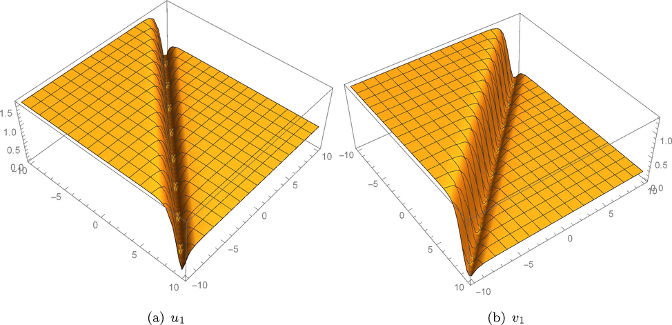

Close

Fig. 1

Solution for (1.3).

Export to PPT

Figures $|u_1|$ and $v_1$ , represent the evolution of the soliton solution corresponding to (1.3), with $a_0(t)=1\text{,}{a}_3(t)=1\text{,}\beta (t)=3\text{,}\alpha (t)=1\text{,}\gamma (t)=1\text{,}(x\text{,}t)\in [-10\text{,}10]\times [-10\text{,}10]$ . In the same way, if we take $G(t)=0$ in (3.10), we obtain solutions to (1.2).Fig. 2.

Close

Fig. 2

Solutions for (1.2).

Export to PPT

Figures $|u_2|$ and $v_2$ , represent the evolution of the soliton solution corresponding to (1.2), with $\delta (t)=1\text{,}\rho (t)=1\text{,}{a}_0(t)=1\text{,}{a}_3(t)=1\text{,}\beta (t)=3\text{,}\alpha (t)=1\text{,}\gamma (t)=1\text{,}(x\text{,}t)\in [-10\text{,}10]\times [-10\text{,}10]$ .Fig. 3.

Close

Fig. 3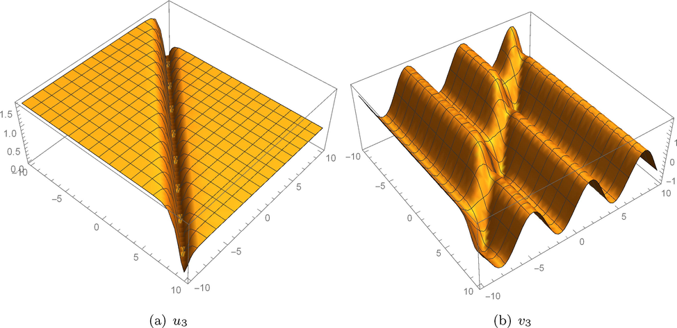

Solutions of (1.1).

Export to PPT

Now, using (3.10) again, we can obtain the following figures, corresponding to solutions of (1.1) in the case that the coefficients are constants, but with a forcing term: Fig. 4.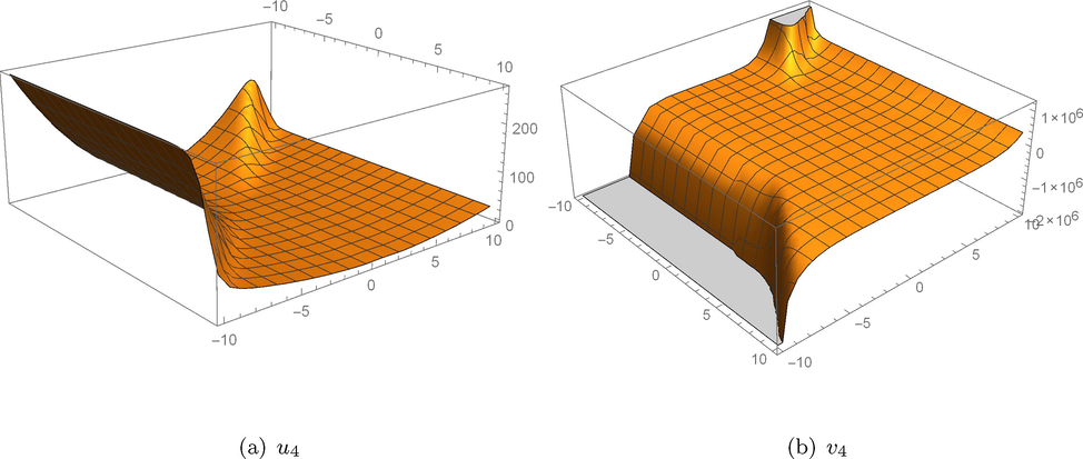

Close

Fig. 4

Solutions to (1.1).

Export to PPT

Figures $|u_3|$ and $v_3$ , represent the evolution of the soliton solution corresponding to (1.1), with $\delta (t)=1\text{,}\rho (t)=1\text{,}{a}_0(t)=1\text{,}{a}_3(t)=1\text{,}\beta (t)=3\text{,}\alpha (t)=1\text{,}\gamma (t)=1\text{,}G(t)=\sin t\text{,}(x\text{,}t)\in [-10\text{,}10]\times [-10\text{,}10]$ .

Now, using variable coefficients and forcing term, we have the following figures:

Figures $|u_4|$ and $v_4$ , represent the evolution of the soliton solution corresponding to (1.1), corresponding to following values: $\delta (t)=t\text{,}\rho (t)=t^3\text{,}{a}_0(t)=1\text{,}{a}_3(t)=1\text{,}\beta (t)=3\text{,}\alpha (t)=1\text{,}\gamma (t)=1\text{,}G(t)=\sin t\text{,}(x\text{,}t)\in [-10\text{,}10]\times [-10\text{,}10]$ .

5 Conclusions

A new model with variable coefficients and forcing term have been studied from the point of view of it traveling wave solutions. Exact solutions for it have been derived by means of the improved tanh-coth method. As a consequence, new exact solutions for the classical Higgs Eq. (1.2), (1.3) have been obtained. We have showed that the used method here, is more general that the Exp $-(\mathrm{\Phi }(\xi ))$ -method and that the $\frac{G^{\prime }(\xi )}{G(\xi )}$ -method used by several authors to handle (1.2) and (1.3). With the aim of make a comparison between the two models (variable coefficients and constants coefficients) we have made the graph of solutions in both cases. The solution are stable, at least, in the intervals considered for its graphs.

References

- Soliton, Nonlinear Evolution Equations and Inverse Scattering. New York: Cambridge University Press; 1991.
- Exact Solutions to the (2+ 1)-Dimensional Boussinesq Equation via Exp -Expansion Method. J. Sci. Res.. 2015;7(3):1-10.
- [Google Scholar]
- Exact traveling wave solutions to the (3+1)-dimensional mKdV-ZK and the (2+1)-dimensional Burgers equations via Exp -expansion method. Alexandria Eng. J.. 2015;54(3):635-644.
- Analytical and Traveling Wave Solutions to the Fifth Order Standard Sawada-Kotera Equation via the Generalized Exp -Expansion Method. J. Appl. Math. Phys.. 2016;04(2) Article ID: 63627, 10 pages
- Symbolic computation of exact solutions expressible in hyperbolic and elliptic functions for nonlinear PDFs. J. Symbolic Compt.. 2004;37(6):669-705. Prepint version: nlin.SI/0201008(arXiv.org)
- Exact solutions of nonlinear Schrödinger’s equation with dual power-law nonlinearity by extended trial equation method. Waves in Raadom and Complex Media. 2014;24(4):439-451.
- Link betwen solitary waves and projective Riccati equations. J. Phys. A Math.. 1992;25:5609-5623.
- Extended tanh-function method and its applications to nonlinear equations. Phys. Lett. A. 2000;227:212-218.
- The Cole-Hopf transformation and improved tanh-coth method applied to new integrable system (KdV6) Appl. Math, and Comp. 2008:957-962.
- [CrossRef] [Google Scholar]
- Special symmetries to standard Riccati equations and applications. Appl. Math, and Comp.. 2010;216(10):3089-3096.
- Exact solutions to the (3+1)-dimensional coupled Klein-Gordon-Zakharov equation using Exp -expansion method. Alexandria Eng. J.. 2016;52(2):1635-1645.
- New Exact Traveling Wave Solutions to the (1+1)-Dimensional Klein-Gordon-Zakharov Equation for Wave Propagation in Plasma Using the Exp -Expansion Method. Propulsionn Power Res.. 2015;4(1):31-39.
- Traveling wave solutions for some important coupled nonlinear physical models via the coupled Higgs equation and the Maccari system. J. King Saud Univ. Sci.. 2015;27:105-112.
- Exp-function method for nonlinear wave equations. Chaos, Solitons & Fractals. 2006;530:700-708.
- Direct methods in Soliton Theory. Berlin: Springer; 1980.
- Homoclinic orbits for the coupled Schrodinger-Boussinesq equation and coupled Higgs equation. J. Phys. Soc. Jpn.. 2003;72(1):189-190.
- Exact solutions of the coupled HIggs equation and the Maccary system using He’s semi-inverse method and -expansion method. Comput. Math. Appl.. 2011;62:2177-2186.
- Coupled Higss field equation and Hamiltonian amplitude equation: Lie classical approach and -expansion method. Pramana-J. Phys.. 2012;79(1):41-60.
- Yang, The applications of bifurcation method to a higher-order KdV equation. Math. Anal. Appl.. 2012;275:1-12.
- Analytical treatment of the coupled Higgs equation and Macary system via exp-function method. Acta Univ. Apulensis. 2013;33:203-216.
- The Korteweg-de Vries equations and generalizations. A remarkable explicit nonlinear transformation. J. Math. Phys.. 1968;9:1202-1204.
- Auto-Bäcklund transformation, Lax Pairs Painlevé property or a variable coefficient Korteweg-de Vries equation. J. Math. Phys.. 1986;27:2640-2646.
- Applications of Lie Group to Differential Equations. Springer-Verlag; 1980.
- New Exact solutions of the generalized Zakharov-Kuznetzov modified equal-with equation. Pramana-J. Phys.cs. 2014;82(6):949-964.
- On N-soliton solutions of coupled Higgs field equation. J. Phys. Soc. Jpn. 1983;52:2277.
- Bifurcations of traveling wave solutions for the coupled Higgs field equation. Int. Journal. of Dif. Eqs. 2011 Article ID 547617, 8 pages
- The tanh-coth method for solitons and kink solutions for nonlinear parabolic equations. Appl. Math. Comput. 2007;188 1467–1074
- The Riccati equation with variable coefficients expansion algorithm to find more exact solutions of nonlinear differential equation. Comput. Phys. Comm.. 2003;152(1):1-8. Prepint version available at http://www.mmrc.iss.ac.cn/pub/mm22.pdf/20.pdf
- A New Sine-Gordon Equation Expansion algorithm to investigate some special nonlinear equations. MMRes.prepint Acad. Sinica. 2004;23:300.