Estimating the probability distribution of the exchange rate between Ghana Cedi and American dollar

Solomon Sarpong

doi:10.1016/j.jksus.2018.04.023

View/Download PDF

Buy Reprints

PDF

Translate this page into:

Original article

31 (

); 177-183

doi:

10.1016/j.jksus.2018.04.023

Estimating the probability distribution of the exchange rate between Ghana Cedi and American dollar

Solomon Sarpong

Department of Statistics, Faculty of Mathematical Sciences, University for Development Studies, Navrongo Campus, Ghana

Received: 2017-12-8, Accepted: 2018-4-16, Published: 2018-04-01

Disclaimer:
This article was originally published by Elsevier and was migrated to Scientific Scholar after the change of Publisher.

Peer review under responsibility of King Saud University.

Abstract

The aim of this research is to find the best probability distribution function (PDF) that fits the data on exchange rate between the Ghana Cedi and American dollar. Economic data in recent times is of much importance to many persons as well as the managers of a country as a whole. Volatilities in these data to a large extent have significant effect on the individuals and the country. The interest in exchange rate volatility by researchers can be attributed to the fact that, it is empirically difficult to predict future exchange rates precisely. The volatility of the US dollar/Ghana Cedi exchange rate is high. This has necessitated the need to have a reliable method for evaluating and minimizing the risk of trading in these currencies. Knowing the type of distribution the exchange rate between the two currencies follow will give stakeholders adequate information to prevent future shocks and loses from any volatility. The data used in this research was the monthly exchange rate between the Ghana Cedi and the American dollar from the year 2000 to 2017. From the analysis, it was observed that the data follow the lognormal distribution. Hence, this analysis has shown that the exchange rate between the Ghana Cedi and the US dollar is best modeled by the lognormal distribution. The Lognormal distribution gives a very good fit to the distribution of the Ghana Cedi and the American dollar.

Keywords

Exchange rate

Forecast

Lognormal distribution

Model

Simulation

Volatility

Show Related Articles from PubMed

1 Introduction

Foreign exchange rate between two currencies specifies how much one currency is worth in terms of the other. A correct or appropriate exchange rate has been one of the most important factors for the growth in the economy of many countries. Exchange rate has direct influence on employment, trade flow, balance of payment, the arrangement of production and consumption, as well as outside loans of a country, Aron et al. (1998).

The world is now a global village hence, the events at one end of the globe affects the others at the extreme end. Individuals and nations trade among themselves. Since the various countries have their own currencies, trading is done in a common currency to facilitate the smoothness of the trade. Since 1944 (Bretton Woods Agreement), the American dollar has been accepted as the currency for international trade. Ghana for that matter also trades with other countries using the American dollar. There have been a lot of volatilities in the exchange rate between the Ghana Cedi and the American dollar. These volatilities have dire consequences on the economy of Ghana. The interest in exchange rate volatility by researchers can be attributed to the fact that, it is empirically difficult to predict future exchange rates precisely.

Many researchers use Box-Jenkins methodology of time series for modeling and forecast. Using Box-Jenkins methodology for forecasting has its deficiencies. This methodology assumes that there is the existence of linear relationship between the variables. But in real-world, time series data are often nonlinear, Lin et al. (2012), Huang et al. (2010), Ding et al. (2009) and Gradojevic and Yang (2006). Secondly, using the Box-Jenkins methodology for model selection procedure depends greatly on the competence and experience of the researchers, Ridhwan et al., 2015.

Hence, using the Box-Jenkins methodology for modeling and forecasting does not give enough accuracy. It is in lieu of this, this paper investigated the type of PDF that the data follows. PDFs are based on the actual data, hence are forward-looking. Also, they do not require a long historical time series in order to be estimated accurately, and furthermore are instantly capable of reflecting a change in the data. Furthermore, PDFs are well-suited for capturing the uncertainty inherent in the data. PDFs are relatively free of mathematical priors Chang and Melick (1999).

Using high-frequency data on Deutschemark and Yen returns against the dollar, Andersen et al., 2001 constructed model-free estimates of daily exchange rate volatility and correlation that cover an entire decade. Their observations included simple normality-inducing volatility transformation, high contemporaneous correlation across volatilities, high correlation between correlation and volatilities, pronounced and persistent dynamics in volatilities and correlations, evidence of long-memory dynamics in volatilities and correlations, and remarkably precise scaling laws under temporal aggregation.

Carroll (2014) found that taking a Bayesian approach, using Markov Chain Monte Carlo (MCMC) and relying on the well-known close relationship between Bayesian posterior means and maximum likelihood, the latter not computationally feasible was able to develop standard errors using balanced repeated replication, a survey-sampling approach. Fujihara and Park (1990) observed that, foreign exchange rate that are unconditional distribution of future prices change measured at high frequency (daily/weekly) has greater area in the tail relative to the normal distribution. However, at a relatively low frequency (monthly/quarterly), the unconditional distribution appears to fit the normal distribution fairly well.

Akgiray and Booth (1987) in their research on the compound distribution models of stock returns: an empirical comparison observed that the distribution of monthly returns can be safely assumed to be approximately normally distributed. Empirical studies by Tucker and Pond (1988) noted that, distribution of exchange returns are long tailed and leptokurtic to satisfy normality. Four processes were investigated in order to find their potential model. They observed discontinuity in the exchange rate and nonstationary sample in their economic appeal. The result favored mixed jump model for all six major trading currencies tested.

In an attempt to fit different PDFs to the data on the daily percentage returns of the Standard & Poor’s (S&P 500), the t-distribution with location/scale parameters was shown to be an excellent choice, Egan (2007). The assumption that daily stock returns are normally distributed has long been disputed, Aparicio and Estrada, 1996. Daily stock returns typically have non-normal and asymmetric distributions (Fama, 1976; Brooks, 2002) no matter how large the data is (Amado, 2002; Brooks, 2002; Bai et al., 2003; Corrado and Zivney, 1992 ). From the research work done on exchange rate between different currencies, it has been observed that the distribution of exchange rate is non-normal and asymmetric. Hence, this research seeks to find the PDF that the exchange rate between the American dollar and Ghana Cedi follow. With the PDF known, more accurate and adequate forecasting can be done.

2 Materials and methods

Some PDFs will be reviewed in order to test the one that best fits the data on exchange rate between the American dollar and the Ghana Cedi.

2.1

2.1 Weibull distribution function

The random variable $X$ is a Weibull distribution with parameters $α > 0, β > 0$ if the pdf of $X$ is given by

(1)

f (X, α, β) = \{\begin{matrix} \frac{α}{β^{α}} x^{e} α - 1 α, & x \geq 0 \\ 0, & x < 0 \end{matrix}

This distribution has an expectation of $E (X) = β (1 + 1 α)$ and a variance $Var (X) = β^{2} \{(1 + 2 α - [{(1 + 1 α)}^{2}]\}$ .

2.2

2.2 Gamma distribution function

A continuous random variable X has the standard Gamma distribution function with parameters $α > 0 and λ > 0$ if its probability distribution function is given by

$f (X) = \{\begin{matrix} \frac{1}{(α)} λ^{α} x^{α - 1} e^{- λ x}, & x > 0 \\ 0, & otherwise \end{matrix}$ . The Gamma distribution function has an expectation, $E (X) = λ$ and variance, $Var (X) = λ$ .

2.3

2.3 Exponential distribution function

The random variable $x$ is an exponential probability distribution function with location and scale parameter $μ$ and $β$ respectively if $f (X) = \frac{1}{β} e^{\frac{- (x - μ)}{β}, x \geq μ; β > 0}$ . The exponential distribution function has an expectation, $E (X) = β$ and variance, $Var (X) = β$ .

2.4

2.4 Lognormal distribution function

A non-negative random variable $X$ is said to have a lognormal distribution if the random variable $y = \ln (x)$ has a normal distribution. The resulting PDF of the lognormal random variable when $\ln (x)$ is normally distributed with parameters $μ$ and $σ$ is given by; $f (X; μ, σ) = \{\begin{matrix} 1 \sqrt{2 π} σ x \sqrt{2 π} σ {xe}^{- \frac{{[\ln (x) - μ]}^{2}}{2 σ^{2}}}, & x \leq 0 \\ 0, & x < 0 \end{matrix}$

The probability distribution function curve is as shown in Fig. 4. The expectation and the variance of the Lognormal distribution are given by; $E (X) = e^{(μ + σ^{2} 2 / 2)}$ and $Var (X) = e^{[2 (μ + σ^{2})]} - e^{(2 μ + σ^{2})}$ respectively.

2.5

2.5 Akaike and Bayesian information criteria

These information criteria were used to compare the distribution that best fits the data. Even though both Akaike and Bayesian information criteria helps in obtaining the best model, each of these try to balance model fit and parsimony of variables and penalizes differently for the number of parameters. In order to get the best model fit, both statistics will be used.

2.6

2.6 Measuring information lost using Kullback-Leibler divergence

In quantifying how much information is in a data, the entropy for the probability distribution is calculated. The entropy probability distribution is given by

$H = - \sum_{i = 1}^{N} p (x_{i}) logp (x_{i})$

By modifying this equation gives the Kullback-Leibler divergence. The Kullback-Leibler divergence gives exactly how much information is lost when a probability distribution is approximated by another. Kullback-Leibler divergence is given by

$D_{KL} (p | | q) = \sum_{i = 1}^{N} p (x_{i}) \log \frac{p (x_{i})}{q (x_{i})}$ where $p (x_{i}) and q (x_{i})$ are the real and approximate probability distributions respectively. The smaller Kullback-Leibler divergence value, the better it is. A smaller Kullback-Leibler divergence value is, the less information is lost in using that probability distribution as an approximation to a data.

2.7

2.7 Gaussian mixture models

This is a probability distribution that consists multiple probability distributions. For d dimensional Gaussian distribution of a vector $X = {(x^{1}, x^{2}, \dots, x^{d})}^{T}$ is defined by $N (x | μ, Σ) = \frac{1}{{(2 π)}^{d / 2} \sqrt{| Σ |}} \exp (- \frac{1}{2} {(x - μ)}^{T} Σ^{- 1} (x - μ))$ ; where $μ$ is the mean and Σ is the variance-covariance matrix. Gaussian Mixture Models tend to find k clusters in a data by minimizing $\frac{{(x - μ)}^{2}}{σ^{2}}$ .

3 Results and discussions

The data was the monthly exchange rate of the Ghana Cedi and the American dollar from the year 2000 to 2017. However, only the data from 2000 to 2015 was used as the training data and data from 2016 to 2017 was used for the validation of the model. During the period understudy, the exchange rate between GHS 0.99–GHS 6.67 to the dollar with a mean of 2.95 (standard error, 0.10).

The quest for this paper is to find a PDF that best approximates the data. In order to do this, a plot of the empirical density and the cumulative distributions of the data were made. From the empirical probability density function in Fig. 1, it was observed that the graph tails off to the right. Hence, the data is positively skewed.

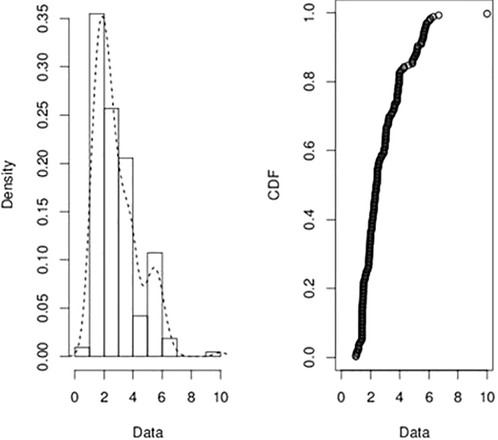
The empirical density (left) and Cumulative distribution function (right) plots for the exchange rate between the Ghana Cedi and the American dollar.

The bootstrapping technique was used in our quest to obtain the Cullen and Frey graph, Fig. 2. From this Figure it was observed that, several distributions were possible fit for the data. From the summary statistics in the Cullen and Frey graph, it was observed that the skewness was positive, 1.23 and kurtosis was 4.81. Hence, the right tail of the data is heavier than the left tail and the data is leptokurtic. These statistics indicate that the possible PDF is positively skewed. As shown in Fig. 2, the distributions in the data include: Weibull, Gamma, Exponential, Logistic and Lognormal, normal, and Beta. However, Fig. 3 shows the distributions with positive skewness. Hence, only the Weibull, Gamma, Exponential and the lognormal distributions will be investigated in order to verify if the data follows any of these distributions.

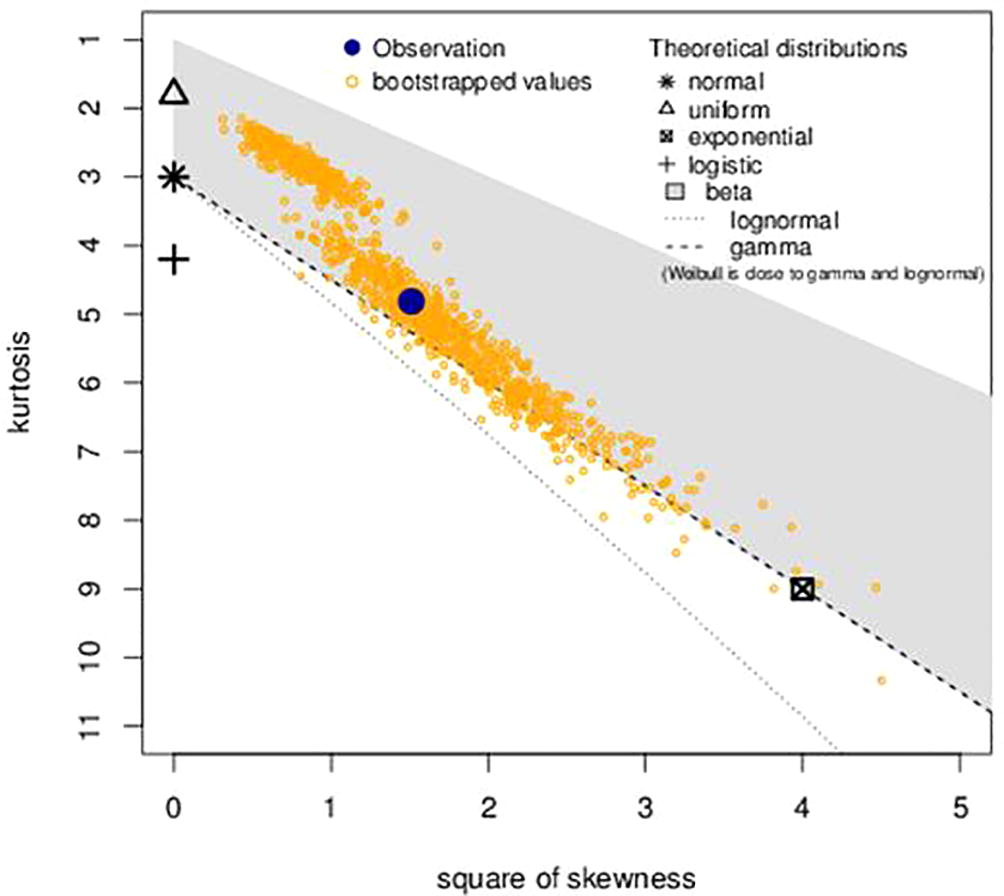
Skewness and Kurtosis plot for the exchange rate between the Ghana Cedi and the American dollar.

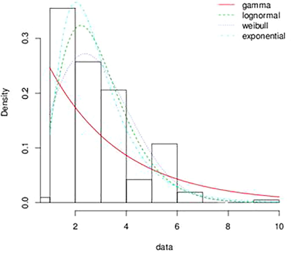
A plot of the histogram and theoretical densities for the exchange rate between the Ghana Cedi and the American dollar.

Fig. 4 shows the theoritical Q-Q plots for the various positively skewed PDFs under consideration. This plot indicates which distribution function the data is more likely to follow. It can be seen that, Gamma distribution deviates remarkable from the hypothetical distribution. Hence, the likely distribution can either be a Weibull, lognormal or exponential distribution. This is also confirmed in the empirical and theoretical cumulative distribution function plot in Fig. 5 and P-P plot in Fig. 6.

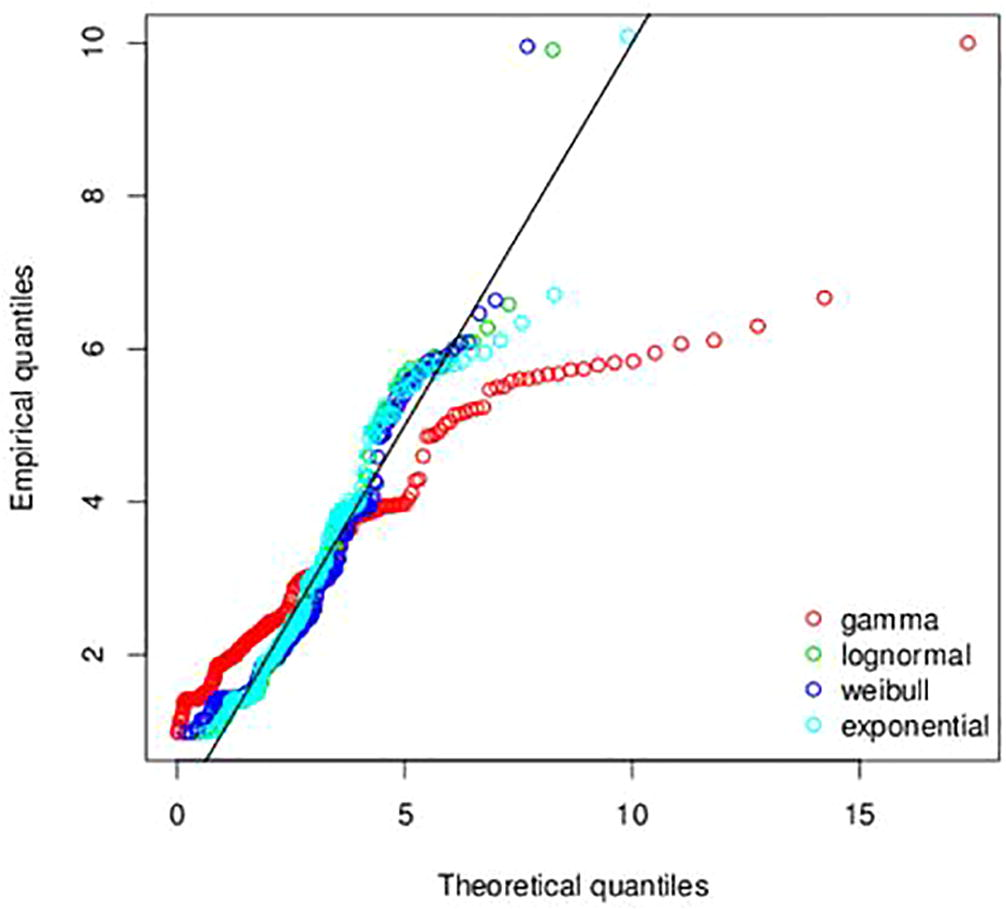
QQ-plot for the exchange rate between the Ghana Cedi and the American dollar.

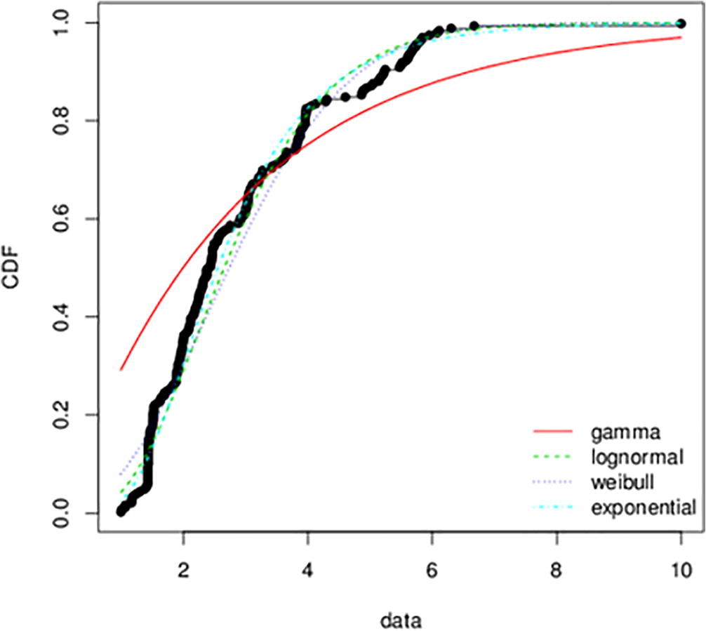
Empirical and theoretical cumulative distributions functions for the exchange rate between the Ghana Cedi and the American dollar.

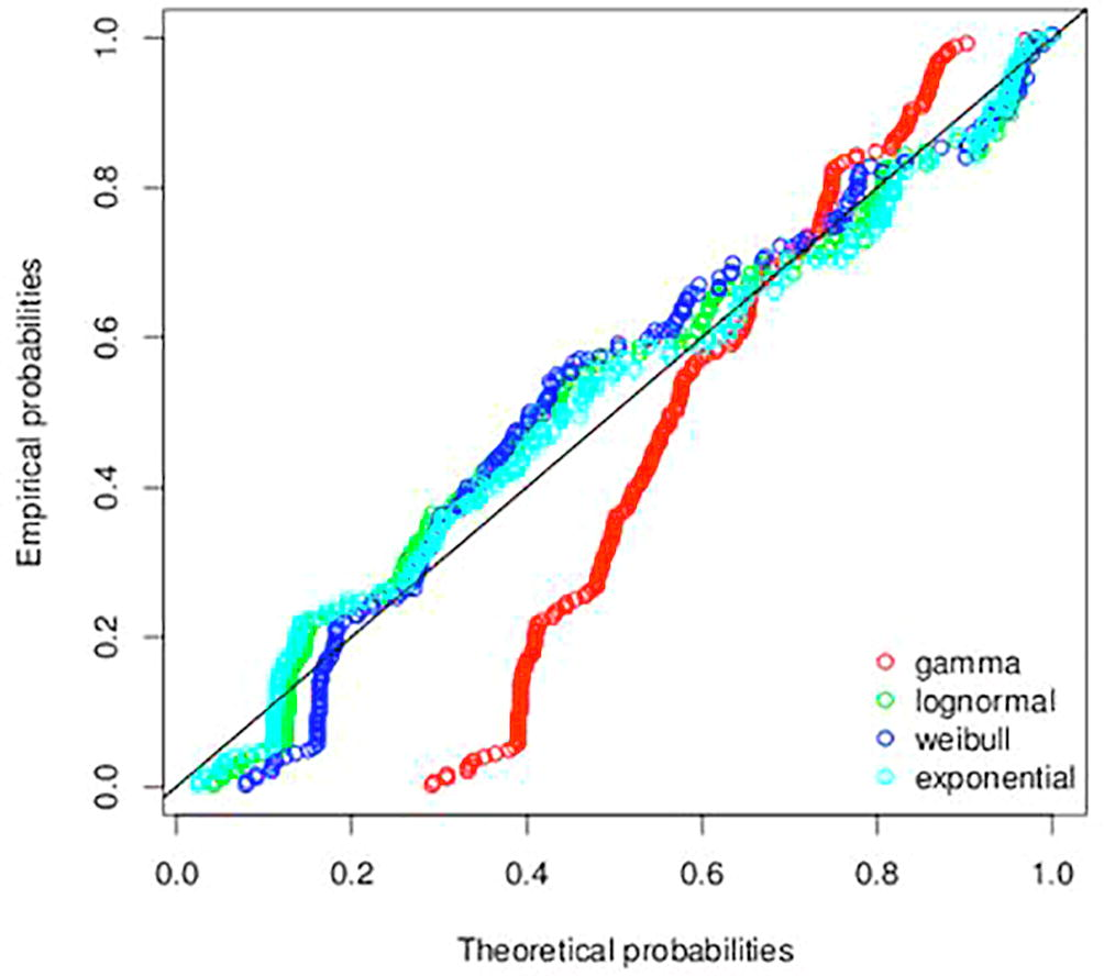
P-P plot of the exchange rate between the Ghana Cedi and the American dollar.

The goodness-of-fit criteria were used to ascertain the best distribution that fits the data. The statistics that were used include log-likelihood, Bayesian and Akaike’s information criteria. The best distribution is the one that has the lowest values for these statistics. From Table 1, it can be observed that lognormal distribution has the lowest values for all these statistics. Hence, the data is likely to be lognormally distributed.

Table 1 The Goodness-of-fit Criteria for the exchange rate between the Ghana Cedi and the American dollar.

Probability Distribution	Akaike’s Information Criterion	Bayesian Information Criterion
Weibull	735.5650	742.3284
Gamma	711.2458	717.9778
Lognormal	697.5699	704.3018
Exponential	880.9186	884.2846

The goodness-of-fit statistics were used to test whether the data is actually lognormally distributed. The Kolmogorov-Smirnov, Cramer-von Mises and Anderson-Darling statistics were used. From the analysis and based on these statistics, it was observed that the data follows the Lognormal distribution. Hence, it has been shown that the exchange rate between the Ghana Cedi and the American dollar follows the Lognormal distribution. It was observed that, this Lognormal distribution has a log-mean value of 0.94 and log-standard deviation of 0.48.

In order to confirm that our data follows the Lognormal distribution, data was generated from simulated Lognormal distribution. The simulated Lognormal distribution has a logmean value of 0.91 and log standard deviation of 0.46. The simulated Lognormal data was then compared with the original data (the exchange rate between the Ghana Cedi and the American dollar). Fig. 7 show plots of the original data on the exchange rate between the Ghana Cedi and the American dollar. Fig. 8 also show the plots from the simulated lognormal data. From Figs. 7 and 8, it can be observed that the two datasets have similar properties. Fig. 9 also shows the plot from these two datasets. From these graphs in Figs. 7–9 , it can be observed that the two datasets are comparable with each other. From the empirical and theoretical cumulative distribution function the Q-Q and P-P plots, almost all the points lie along the fitted curve. Hence, the Lognormal distribution is the best fit for the data.

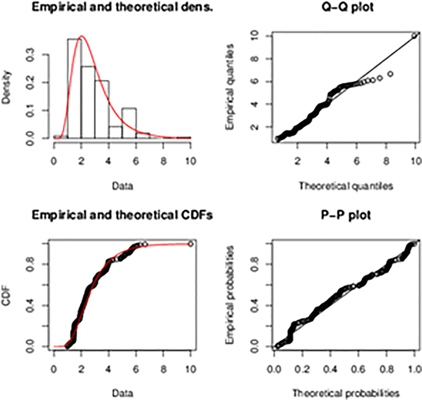
Plots of the original data on the exchange rate between the Ghana Cedi and the American dollar.

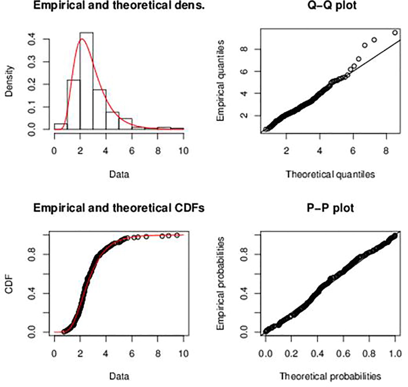
Plots of the simulated data of the exchange rate between the Ghana Cedi and the American dollar.

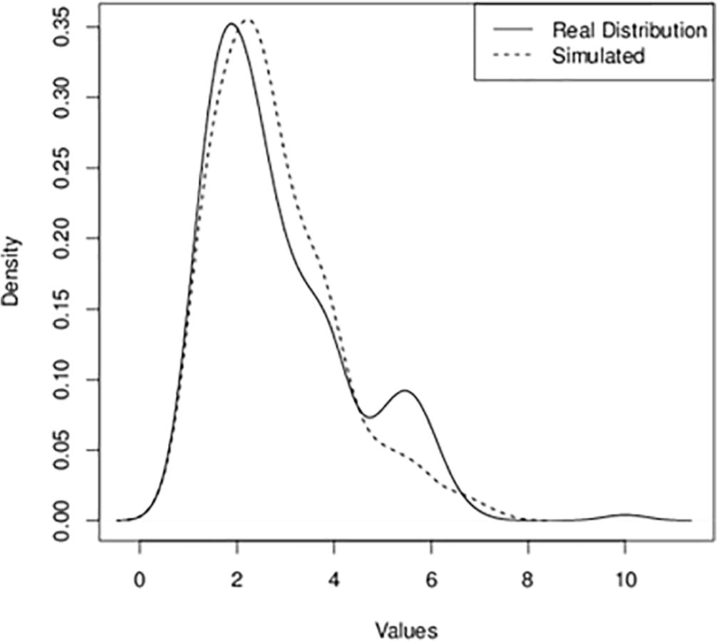
A graph of the distribution of real and simulated exchange rate between the Ghana Cedi and the American dollar.

The Wilcoxon signed rank test with continuity correction was conducted to test if the two datasets have the same distribution or not. From the test, it was observed that there was a p-value of 0.4132. Hence with a significance level of 0.05, it can be observed that the two datasets are identical. It can therefore be concluded that the original data on the exchange rate between the Ghana Cedi and the American dollar follows the Lognormal distribution.

One way of judging a derived probability density function is its empirical performance – i.e. its ability to predict accurately, Chang and Melick (1999). Hence, in order to verify the practicability of using the lognormal distribution for forecasting, how best the simulated data approximates the original data was investigated. In order to do this, the Lognormal distribution was used to forecast the exchange rate between the Ghana Cedi and American dollar from 2016 to 2017. The forecast data was compared with the remaining of the original data (2016–2017). The comparison was done using two sample t-test. From the analysis, the t-value was −32.42, p-value = 0.12. Hence, it can be seen that there is no difference in the values from the two distributions.

To further check the adequacy of the fitted probability distribution, the autocorrelation of the errors of both the real and simulated probability distributions were analyzed. Figs. 10 and 11 shows the autocorrelation of the errors for the real and simulated probability distributions respectively.

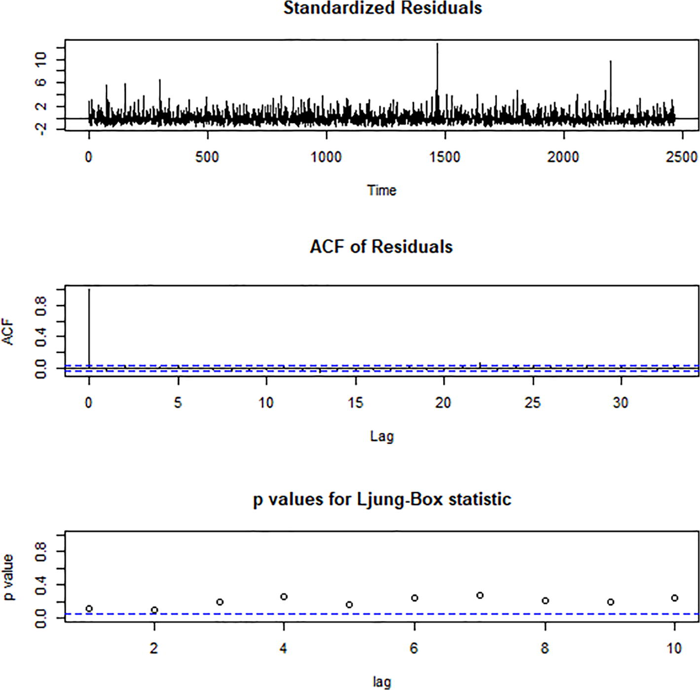
The autocorrelation of the errors for the real probability distribution.

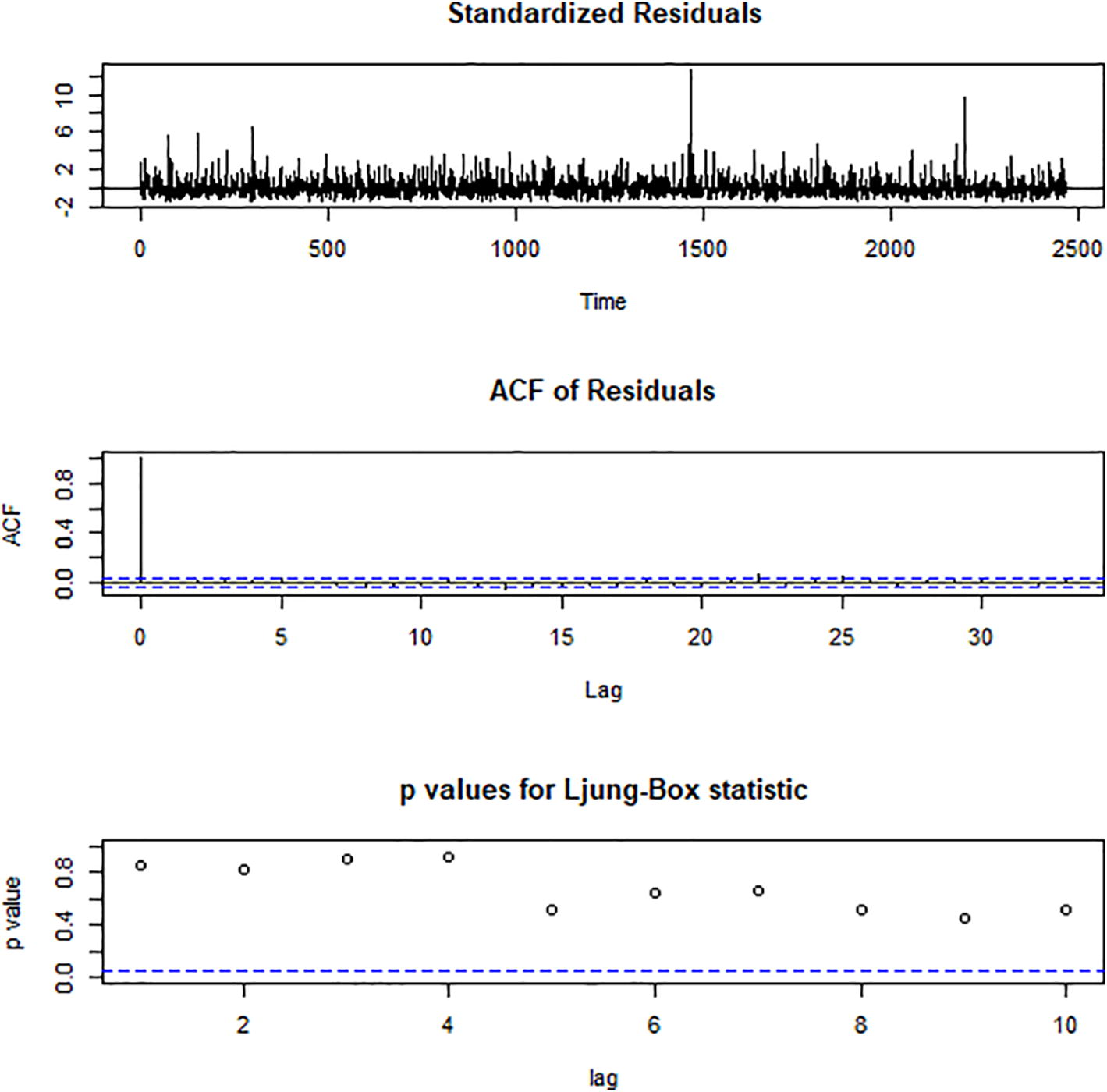
The autocorrelation of the errors for the simulated probability distribution.

The Box-Ljung test shows that the autocorrelations among the errors for the real probability distribution are zero (p-value = 0.30). This indicates that the errors are random and that the probability distribution provides an adequate fit to the data. Likewise, the Box-Ljung test shows that the autocorrelations among the errors for the simulated probability distribution are zero (p-value = 0.43). This indicates that the errors are random and that the log-normal probability distribution provides an adequate fit to the data. Furthermore, the Kullback-Leibler divergence was calculated to assess the amount of information lost when any of the probability distributions was used to approximate the data. Table 2 show the probability distributions and the corresponding Kullback-Leibler divergence values calculated. It can be observed that, less amount of information is lost when the lognormal probability distribution is used to approximate the data.

Table 2 The Kullback-Leibler divergence values for the exchange rate between the Ghana Cedi and the American dollar.

Probability distribution	Kullback-Leibler divergence
Weibull	0.65
Gamma	0.79
Lognormal	0.26
Exponential	0.63

3.1

3.1 Gaussian mixture models

Table 3 shows the summary statistics of the three possible clusters in the data. It can be observed that, when the data is considered to be a single cluster, the log-likelihood, Bayesian Information Criterion and Integrated Complete-data Likelihood had the highest values. This implies that, in spite of the fact that the data maybe having some clusters inherent in it, the data is well represented when it is assumed that the data has only one cluster.

Table 3 Summary statistics for Gaussian mixture model.

Number of clusters	Log-likelihood	Bayesian information criterion	Integrated complete-data likelihood
1	−5186.83	−10389.28	−10389.3
2	−5038.97	−10116.99	−10347.7
3	−4929.5	−9921.51	−10327.8

4 Conclusion

The sole aim of persons who deal in exchange of currencies is to minimize loss through the volatilities in the exchange rates between the currencies. Hence, being able to forecast accurately the exchange rate maximizes the returns in profit. Hence, this research has adequately proved that the exchange rate between the Ghana Cedi and the American dollar follows the lognormal distribution. By using the Lognormal distribution in predicting the possible exchange rate between the two currencies will result in maximum returns in profit. From the autocorrelation of the errors of both the real and simulated probability distributions in addition to the Box-Ljung test, it was observed that the errors are random. The randomness of the autocorrelation of the errors shows that the fitted distribution adequately fits the data. From the Kullback-Leibler divergence values calculated, it can be observed that, there is less loss of information when the lognormal probability distribution is used to approximate the data than the other probability distributions. Hence, the lognormal probability distribution better approximates the data.

References

Akgiray V., Booth G.G., . Compound distribution models of stock returns: an empirical comparison. J. Fin. Res.. 1987;10(3):269-280.
[Google Scholar]
Amado P., 2002. Skewness in Individual Stocks at Different Investment Horizons, 2 Quantitative Finance 139.
Andersen T.G., Diebold F.X., Bollerslev T., Labys P., . The distribution of realized exchange rate volatility. American statistical association. J. Am. Stat. Assoc.. 2001;96(453) Applications and Case Studies
[Google Scholar]
Aparicio F. M. and Estrada J., 1996. Empirical distributions of stock returns: Scandinavian securities markets, 1990-95. Departamento de Estadística Working Papers 1996-10. Statistics and Econometrics. Universidad Carlos III de Madrid.
Aron J., Elbadawi I., Kahn B., . Determinants of the real exchange rate in South Africa, CSAE Working Paper Series 1997-16. In: Centre for the Study of African Economics. University of Oxford; 1998.
[Google Scholar]
Bai X.-Z., Russell J.R., George C., Tiao G.C., . Kurtosis of GARCH and stochastic volatility models with non-normal innovations. J. Econ.. 2003;114(2):349-360.
[Google Scholar]
Brooks C., . Introductory Econometrics for Finance (3rd Edition). Cambridge University Press; 2002.
Corrado C.J., Zivney T.L., . The specification and power of the sign test in event study hypothesis tests using daily stock returns. J. Fin. Quantit. analysis. 1992;27(3):465-478. Cambridge University Press
[Google Scholar]
Carroll R.J., . Estimating the distribution of dietary consumption patterns. Stat Sci.. 2014;29(1):2-8.
[Google Scholar]
Chang P.H.K., Melick W.R., . Workshop on estimating and interpreting probability density functions. Bank for Intrnational Settlements Information. Press Library Serv. 1999:1-10.
[Google Scholar]
Ding Y., Li S., Li L., . An analysis on chaos behavior of currency exchange rate undulation. Wuhan, Hubei: First International Workshop on Education Technology and Computer Science; 2009. p. :599-602.
Egan W. J., 2007. The Distribution of S&P 500 Index Returns.
Fama E.F., . Foundations of finance. J. Fin.. 1976;38:143-145.
[Google Scholar]
Fujihara R., Park K., . The probability distribution of future price in the foreign exchange market: a comparison of candidate processes. J. Future Markets. 1990;10(6):623-641.
[Google Scholar]
Gradojevic N., Yang J., . Non-linear, non-parametric, non-fundamental exchange rate forecasting. J. Forecast. No.. 2006;25:227-245.
[Google Scholar]
Huang S.C., Chuang P.J., Wu C.F., . Chaos-based support vector regressions for exchange rate forecasting. Expert Syst. Appl.. 2010;37(12):8590-8598.
[Google Scholar]
Lin C.-S., Chiu S.-H., Lin T.-Y., . Empirical mode decomposition-based least squares support vector regression for foreign exchange rate forecasting. Econ. Model.. 2012;29:2583-2590.
[Google Scholar]
Radhwan A., Kamel M., Dahab M.Y., Hassanien A., . Forecasting exchange rates: a chaos-based regression approach. Int. J. Rough Sets Data Analysis. 2015;2(1):38-57.
[Google Scholar]
Tucker A.L., Pond L., . The probability distribution of foreign exchange price changes: test of candidate processes. Rev. Econ. Stat.. 1988;70(4):638-647.
[Google Scholar]