

Enhancing hyperspectral remote sensing image classification using robust learning technique
-
Received: ,
Accepted: ,
This article was originally published by Elsevier and was migrated to Scientific Scholar after the change of Publisher.
Peer review under responsibility of King Saud University.
Abstract
Advanced sensor tech integrates into diverse applications, including remote sensing, robotics, and IoT. Combining artificial intelligence (AI) with sensors enhances their capabilities, creating smart sensors, revolutionizing remote sensing and Internet of Things (IoT). This synergy forms a potent technology in the field. This study carries out a comprehensive analysis of the progress made in Hyperspectral sensors and AI-based classification techniques that are employed in remote sensing fields that utilize hyperspectral images. The classification of images obtained from Hyperspectral Sensors (HSS) has emerged as a prominent research subject within the domain of remote sensing. HSS offer a wealth of information across numerous spectral bands, supporting diverse applications such as land cover classification, environmental monitoring, agricultural assessment, change detection, and more. However, the abundance of data present in HSS also poses the challenge called the curse of dimensionality. The reduction of data dimensionality is crucial before applying any machine learning model to achieve optimal results. The present study introduces a new hybrid strategy combining the Back-Propagation algorithm with a variable adaptive momentum (BPVAM) and principal component analysis (PCA) for the purpose of classifying hyperspectral images. PCA is first applied to obtain an optimal set of discriminative features by eliminating highly correlated and redundant features. These features are then fed into the BPVAM model for classification. The addition of the momentum term in the weight update equation of the backpropagation algorithm helped achieve faster convergence with high accuracy. The proposed model was subjected to evaluation through experiments conducted on two benchmark datasets. These results indicated that the hybrid model based on BPVAM with PCA is an efficient technique for HSS classification.
Keywords
Backpropagation with variable adaptive momentum
Principal component analysis
Hyperspectral image classification
Dimensionality reduction
Hyperspectral sensors

1 Introduction
The use of AI techniques based on Deep Learning and IoT technologies has brought about a revolutionary period in the discipline of remote sensing. This synergy has not only enabled more sophisticated and efficient data acquisition, analysis, and interpretation but has also marked a transformative phase in remote sensing. The integration of deep learning algorithms empowers the processing of vast datasets with heightened precision and speed, while IoT technologies facilitate real-time monitoring and seamless data transmission, further enhancing the capabilities of remote sensing systems. These advancements have significantly broadened the scope of remote sensing applications and have opened up new avenues of research and development in the field (Anand et al., 2022; Grewal et al., 2023; Firat et al., 2022a, 2022b; Krishna et al., 2022; Li et al., 2022; Liu and Dhakal, 2020; Sharma and Biswas, 2022). IoT plays a critical role in the data collection process for remotely sensed images, resulting in a marked improvement in the accuracy of various classification methods (Sharma and Biswas, 2022; Ullo and Sinha, 2021; Wang et al., 2019). The integration of advanced sensor technology has enabled the acquisition of Hyperspectral Images (HSIs) that possess a high degree of resolution both in the spatial and spectral domains. These images have become a ubiquitous tool in a multitude of domains, ranging from mineral detection to crop evaluation, environmental management, etc. (Liu and Dhakal, 2020; Ullo and Sinha, 2021; Deepa et al., 2023; Grewal et al., 2023; Zhao et al., 2023; Zhou et al., 2023).
Hyperspectral sensors produce images of high-resolution which contain a large set of bands. These images are captured by high-quality sensors that use different spectral frequencies (Elmaizi et al., 2019). For HSS, the wavelength varies between the visible and infrared spectrum (Zhang et al., 2021). HSS provides rich information about the object of interest that can help discriminate a wide range of objects. It is impossible to acquire such a large number of bands with multispectral sensors as they normally capture 3–12 bands (Praveen and Menon, 2021; Zhao et al., 2021). The HSS has been extensively utilized across numerous applications such as change detection (Wen et al., 2021), plant phenotyping (Sarić et al., 2022), tomographic reconstruction (Huang et al., 2022), natural gas leakage identification (Ran et al., 2022), object detection (Wen et al., 2021), etc. This indicates the important role of HSS which can help solve many problems.
While the multitude of spectral bands in hyperspectral data offers valuable insights, it also introduces the challenge of higher dimensionality, which can potentially hinder classifier performance. The data across various bands may exhibit high correlations, noise, or even irrelevance. The presence of such extensive correlated and redundant information not only degrades the performance of the classifier but also amplifies the complexity of processing such voluminous data. It is imperative to address these issues carefully to fully exploit the potential of hyperspectral data for diverse classification tasks.
This paper proposes a hybrid approach for HSS classification, which integrates two techniques: PCA and BPVAM. PCA is a powerful technique used for feature extraction, while BPVAM is used for classification. A variable adaptive momentum term in the BPVAM has improved the performance of the model. This innovative combination is developed to address the challenges in accurately classifying hyperspectral images, which are typically high-dimensional and complex in nature. The BPVAM algorithm allows for the dynamic adjustment of the learning rate throughout the training process, while PCA helps in reducing the dimensionality of the data, thereby simplifying the classification task. The study aims to demonstrate the efficacy of this hybrid strategy in providing more accurate and efficient results compared to traditional approaches. Consequently, the combination of BPVAM and PCA yields a remarkably robust classifier for HSS. It has been shown that the model's performance improves for HSS not only in terms of accuracy but also in terms of faster convergence.
The paper is organized in the following manner: In Section 2, the datasets conducted in the study are presented. The proposed approach is explicated in Section 3. The experimental results are discussed in Section 4. Finally, the paper is completed with a conclusion.
2 Materials
In this study, the effectiveness of the proposed methods was assessed using two widely used hyperspectral datasets, namely the Indian Pines and the University of Pavia datasets. To give a complete understanding of each dataset, the following sections have been dedicated to providing an in-depth explanation of each one of them.
2.1 Indian Pines
The Indian Pines dataset was obtained through the use of an airborne sensor named Airborne Visible/Infrared Imaging Spectrometer (AVIRIS). With dimensions of 145 × 145 pixels and a total of 220 spectral bands, this dataset is a valuable resource for hyperspectral imaging analysis. The wavelength range of the bands spans from 0.4 to 2.5 μm, providing comprehensive spectral information that can be utilized to identify different areas and substances with great precision. The absorption bands are removed for this study, and the remaining 200 bands are used. It consists of sixteen different land cover classes.
2.2 University of Pavia
The University of Pavia dataset encompasses an urban area within the city of Pavia, Italy, and was collected through the application of a Reflective Optics System Imaging Spectrometer (ROSIS-3). It comprises 115 spectral bands with a wavelength range of 0.43–0.86 μm and a spatial resolution of 1.3 m/pixel, represented by 610 × 340 pixels. Despite its high spatial resolution, the dataset contained some noisy channels that were subsequently removed, remaining only 103 channels to be employed in this study for the purpose of classification. It consists of nine land-cover classes.
3 Proposed method
Hyperspectral images contain a huge number of input bands (usually in hundreds). Although these bands provide useful details of the objects of interest, this may also lead to a high correlation between channels. The presence of excessive redundancies can have an adverse impact on the efficacy of the classification technique. This study employs a two-step approach, in which the PCA is initially utilized to reduce the data dimensional, followed by the deployment of the BPVAM to classify each individual pixel within the input image. BPVAM is an improvement of the BP algorithm; therefore, in this section, the BP algorithm is described, first followed by BPVAM, and an introduction to PCA. Finally, we describe the application of these hybrid techniques for HSS classification.
3.1 BPVAM algorithm
To take full advantage of the momentum term, an optimal value of momentum should be selected. A small value may not help take the model out of local minima and a large value can make the model fluctuate around the optimal value. To overcome these issues, an adaptive momentum (
3.2 Principal component analysis (PCA)
PCA, also referred to as Karhunen-Loeve transform, was first proposed by Pearson (Pearson, 1901). The method is a multivariate statistical analysis technique, which effectively reduces the dimensionality of the data through reduction. Its work is started by receiving d-dimensional input vectors. The objective of PCA is to represent these d-dimensional vectors using k-dimensional vectors, where k≪d. It first calculates the mean vector (μ) and covariance matrix Σ using the d-dimensional space. The computation and arrangement of the eigenvalues and their corresponding eigenvectors are performed to allocate the dimensional space with maximal variance. The original data is then transformed using the newly generated Eigenvectors.
3.3 BPVAM-PCA HSS classification
The input data consists of a high number of channels. Before applying the BPVAM algorithm, the utilization of PCA was employed to reduce the dimensional magnitude of the input features. The robustness of the system was improved when highly redundant features with low variance were discarded using PCA. This improved the likelihood of the model reaching convergence early in the training process without affecting its performance.
The original data set for the Indian Pines data consisted of 220 bands, while The University of Pavia consisted of 115 bands. PCA was applied to select the most suitable number of bands to obtain highly discriminative features. We experimented with three different feature sizes for the University of Pavia (5, 10, and 20). Increasing the dimensional beyond 20 did not improve accuracy. Moreover, reducing features below ten also decreased the performance of the model. Similarly, for the Indian pines dataset, we empirically selected feature sizes of 10, 40, and 80. The features that have been selected were then taken as input to the BPVAM model for the classification of each pixel into one of the categories. We observed that the BPVAM reached a low steady-state error faster during training using features with high variance and low autocorrelation.
The workflow of the proposed BPVAM-PCA model will whole steps is illustrated in Fig. 1. The initiation of the learning process involves the random initialization of the weight vectors and other learning parameters of the model. The input data is passed to the PCA algorithm first and then fed it BPVAM model for classification. The training process is iterative over several epochs to obtain optimal values for both weights and biases. Two possibilities are used to stop the training process: maximum number of iterations and stopping criteria. The training will continue until the error reaches the acceptable threshold value or reach the maximum number of iterations. After training is completed, the optimized weights and biases will be stored and taken into consideration for the subsequent stage of processing. Finally, the test data is passed to the trained/optimized model which will then produce the final class labels for each pixel.
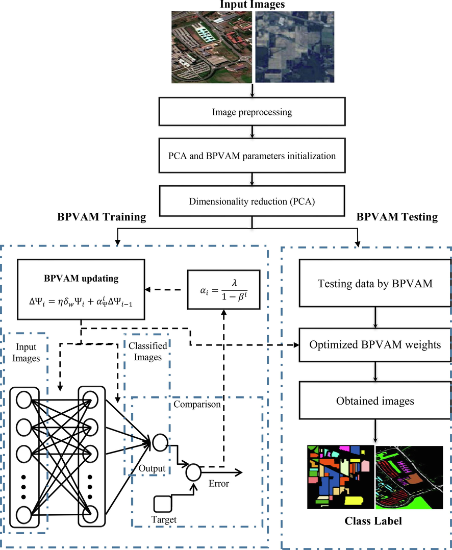
- Block diagram of the BPVAM-PCA method.
4 Experimental results
This section describes the performance evaluation of the proposed method for HSS classification on two well-known benchmark datasets: the Indian Pines and the Pavia University datasets. It is preferable to test data with known characteristics and challenges to assess the level and size of the impact of the proposed model and its ability to achieve competitive results compared to the recently published methods.
The performance of the proposed hybrid BPVAM-PCA is compared with BP, BP-PCA, and BPVAM on both datasets. The number of features for the dimensionality reduction were empirically selected. Therefore, three different experiments were conducted using different sizes of features from PCA to obtain the optimal subset. The datasets were divided into training (75 %) and testing (25 %) subsets. The maximum number of iterations was set to 200 as all evaluated models converged before reaching 200 iterations. The hyperparameters used in this study as follows: for Indian Pines (BP:
4.1 Indian Pines dataset
Table 1 summarizes the quantitative results obtained for the Indian Pines dataset. The best feature sizes used in this dataset for PCA are 10, 40, and 80. It can be seen that the BPVAM-PCA algorithm produced relatively better performance compared to BP-PCA for all three sizes of extracted features. Data with 80 features produced better results with an accuracy of 98.83 % and SSE of 1.1233 for the training dataset, while the accuracy of 97.30 % and SSE of 1.0665 for the testing dataset. The performance of BP-PCA was relatively similar to BPVAM-PCA which achieved accuracy = 0.9869 and error = 1.2350 in training, and accuracy = 96.71 % and SSE = 1.19 in the testing. BPVAM-PCA produces on average 2 % better accuracy for other feature sizes than the BP-PCA algorithm.
| Feature Size | Method | Training | Testing | ||
|---|---|---|---|---|---|
| Accuracy | SSE | Accuracy | SSE | ||
| 10 | BP-PCA | 94.82 | 2.5716 | 88.53 | 2.42 |
| BPVAM-PCA | 96.43 | 2.0408 | 91.00 | 1.90 | |
| 40 | BP-PCA | 97.04 | 1.6328 | 93.39 | 1.56 |
| BPVAM-PCA | 98.23 | 1.4545 | 95.23 | 1.38 | |
| 80 | BP-PCA | 98.69 | 1.2350 | 96.71 | 1.19 |
| BPVAM-PCA | 98.83 | 1.1233 | 97.30 | 1.06 | |
Initially, all models produced higher SSE due to random initialization. As the iterations proceeded, all models started to gradually converge.
In Table 2, Pre, Rec, Spe, and F1 results for two methods, BP-PCA and BPVAM-PCA, are compared across different feature sizes for the Indian Pines dataset with 16 distinct classes. BPVAM-PCA consistently exhibits superior performance over BP-PCA in terms of Pre, Rec, and F1 across most classes and feature sizes. This suggests that BPVAM-PCA not only minimizes false positives and maximizes true positives more effectively but also strikes a better balance between Pre and Rec. Both methods demonstrate high Spe, indicating their proficiency in identifying true negatives among actual negative instances. The overall trend in the results indicates that BPVAM-PCA is better suited for the Indian Pines dataset, delivering more accurate and reliable predictions than BP-PCA.
| Method | Label | Class | Feature Size (10) | Feature Size (40) | Feature Size (80) | |||||||||
|---|---|---|---|---|---|---|---|---|---|---|---|---|---|---|
| Pre. | Rec. | Spe. | F1 | Pre. | Rec. | Spe. | F1 | Pre. | Rec. | Spe. | F1 | |||
| BP-PCA | 1 | Alfalfa | 0.00 | 0.00 | 1.00 | 0.00 | 0.00 | 0.00 | 1.00 | 0.00 | 0.00 | 0.00 | 1.00 | 0.00 |
| 2 | Corn-notill | 0.95 | 0.88 | 0.99 | 0.91 | 0.97 | 0.96 | 1.00 | 0.96 | 0.99 | 0.98 | 1.00 | 0.98 | |
| 3 | Corn-mintill | 0.82 | 0.92 | 0.98 | 0.86 | 0.93 | 0.95 | 0.99 | 0.94 | 0.94 | 0.98 | 0.99 | 0.96 | |
| 4 | Corn | 0.63 | 0.71 | 0.99 | 0.67 | 0.76 | 0.85 | 0.99 | 0.80 | 0.95 | 0.92 | 1.00 | 0.93 | |
| 5 | Grass-pasture | 0.86 | '0.77 | 0.99 | 0.81 | 0.90 | 0.92 | 1.00 | 0.91 | 0.96 | 0.98 | 1.00 | 0.97 | |
| 6 | Grass-trees | 0.91 | 0.99 | 0.99 | 0.95 | 0.94 | 0.96 | 0.99 | 0.95 | 0.98 | 0.98 | 1.00 | 0.98 | |
| 7 | Grass-pasture-mowed | 0.00 | 0.00 | 0.99 | 0.00 | 0.00 | 0.00 | 0.99 | 0.00 | 0.23 | 0.50 | 1.00 | 0.32 | |
| 8 | Hay-windrowed | 0.97 | 0.63 | 1.00 | 0.77 | 0.97 | 0.65 | 1.00 | 0.78 | 1.00 | 0.92 | 1.00 | 0.96 | |
| 9 | Oats | 0.00 | 0.00 | 0.99 | 0.00 | 0.22 | 1.00 | 0.99 | 0.36 | 0.60 | 1.00 | 1.00 | 0.75 | |
| 10 | Soybean-notill | 0.89 | 0.99 | 0.99 | 0.94 | 0.97 | 0.98 | 1.00 | 0.98 | 0.98 | 0.99 | 1.00 | 0.98 | |
| 11 | Soybean-mintill | 0.97 | 0.96 | 0.99 | 0.97 | 0.98 | 0.99 | 0.99 | 0.99 | 0.99 | 0.99 | 1.00 | 0.99 | |
| 12 | Soybean-clean | 0.93 | 0.91 | 1.00 | 0.92 | 0.96 | 0.94 | 1.00 | 0.95 | 0.98 | 0.97 | 1.00 | 0.98 | |
| 13 | Wheat | 0.62 | 0.84 | 0.99 | 0.72 | 0.82 | 0.88 | 1.00 | 0.85 | 0.89 | 0.96 | 1.00 | 0.92 | |
| 14 | Woods | 0.92 | 0.92 | 0.99 | 0.92 | 0.96 | 0.97 | 0.99 | 0.97 | 0.97 | 0.97 | 1.00 | 0.97 | |
| 15 | Buildings-Grass-Trees-Drives | 0.74 | 0.75 | 0.99 | 0.75 | 0.85 | 0.89 | 0.99 | 0.87 | 0.88 | 0.93 | 1.00 | 0.90 | |
| 16 | Stone-Steel-Towers | 0.00 | 0.00 | 1.00 | 0.00 | 1.00 | 0.43 | 1.00 | 0.61 | 0.93 | 0.61 | 1.00 | 0.74 | |
| BPVAM-PCA | 1 | Alfalfa | 0.00 | 0.00 | 1.00 | 0.00 | 0.00 | 0.00 | 1.00 | 0.00 | 0.00 | 0.00 | 1.00 | 0.00 |
| 2 | Corn-notill | 0.96 | 0.92 | 0.99 | 0.94 | 0.98 | 0.96 | 1.00 | 0.97 | 0.98 | 0.99 | 1.00 | 0.99 | |
| 3 | Corn-mintill | 0.87 | 0.94 | 0.99 | 0.90 | 0.92 | 0.97 | 0.99 | 0.94 | 0.96 | 0.98 | 1.00 | 0.97 | |
| 4 | Corn | 0.64 | 0.71 | 0.99 | 0.67 | 0.77 | 0.86 | 0.99 | 0.82 | 0.92 | 0.93 | 1.00 | 0.92 | |
| 5 | Grass-pasture | 0.95 | 0.83 | 1.00 | 0.89 | 0.95 | 0.93 | 1.00 | 0.94 | 0.98 | 0.98 | 1.00 | 0.98 | |
| 6 | Grass-trees | 0.91 | 1.00 | 0.99 | 0.95 | 0.96 | 0.97 | 1.00 | 0.97 | 0.98 | 0.98 | 1.00 | 0.98 | |
| 7 | Grass-pasture-mowed | 0.00 | 0.00 | 0.99 | 0.00 | 0.08 | 0.17 | 1.00 | 0.11 | 0.33 | 0.50 | 1.00 | 0.40 | |
| 8 | Hay-windrowed | 0.99 | 0.82 | 1.00 | 0.89 | 1.00 | 0.89 | 1.00 | 0.94 | 0.98 | 0.95 | 1.00 | 0.97 | |
| 9 | Oats | 0.00 | 0.00 | 1.00 | 0.00 | 0.40 | 1.00 | 1.00 | 0.57 | 0.71 | 0.83 | 1.00 | 0.77 | |
| 10 | Soybean-notill | 0.91 | 0.98 | 0.99 | 0.94 | 0.97 | 0.97 | 1.00 | 0.97 | 0.99 | 0.99 | 1.00 | 0.99 | |
| 11 | Soybean-mintill | 0.98 | 0.97 | 0.99 | 0.97 | 0.99 | 0.98 | 1.00 | 0.99 | 0.99 | 1.00 | 1.00 | 0.99 | |
| 12 | Soybean-clean | 0.92 | 0.91 | 1.00 | 0.91 | 0.95 | 0.97 | 1.00 | 0.96 | 0.99 | 0.97 | 1.00 | 0.98 | |
| 13 | Wheat | 0.62 | 0.82 | 0.99 | 0.71 | 0.85 | 0.90 | 1.00 | 0.88 | 0.91 | 0.96 | 1.00 | 0.93 | |
| 14 | Woods | 0.93 | 0.93 | 0.99 | 0.93 | 0.97 | 0.98 | 1.00 | 0.97 | 0.98 | 0.98 | 1.00 | 0.98 | |
| 15 | Buildings-Grass-Trees-Drives | 0.80 | 0.79 | 0.99 | 0.80 | 0.90 | 0.91 | 1.00 | 0.90 | 0.91 | 0.94 | 1.00 | 0.92 | |
| 16 | Stone-Steel-Towers | 1.00 | 0.26 | 1.00 | 0.41 | 1.00 | 0.65 | 1.00 | 0.79 | 0.94 | 0.65 | 1.00 | 0.77 | |
Fig. 2 shows the convergence behavior of BP-PCA and BPVAM-PCA methods for different feature sizes on the Indian Pines dataset. The visual results confirm the performance of the proposed model shown in Tables 1, and 2 by providing significant performance enhancement for BPVAM-PCA over BP-PCA. The data extracted with 80 features give better results by achieving less error and faster convergence. The improved performance also demonstrates that learning of BPVAM-PCA is robust by dealing with different size and feature characteristics.
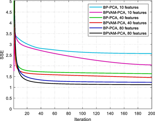
- Convergence behavior of BP-PCA and BPVAM-PCA methods using different features on sthe Indian Pines dataset.
It can be seen from Fig. 2 that both models resulted in relatively higher SSE when the feature size was set to 10. This indicates that dimensionality reduction from large dimensional space to very low dimensional space resulted in the loss of important information. In addition, this also leads the models to converge slowly to reach a steady-error state. Especially, BPVAM-PCA took almost 180 iterations to reach a stable error state. For features sizes of 40 and 80, the overall behavior of the models was similar. It can be noticed that BPVAM-PCA not only converged faster but also resulted in lower SSE from the very beginning till the end of iterations.
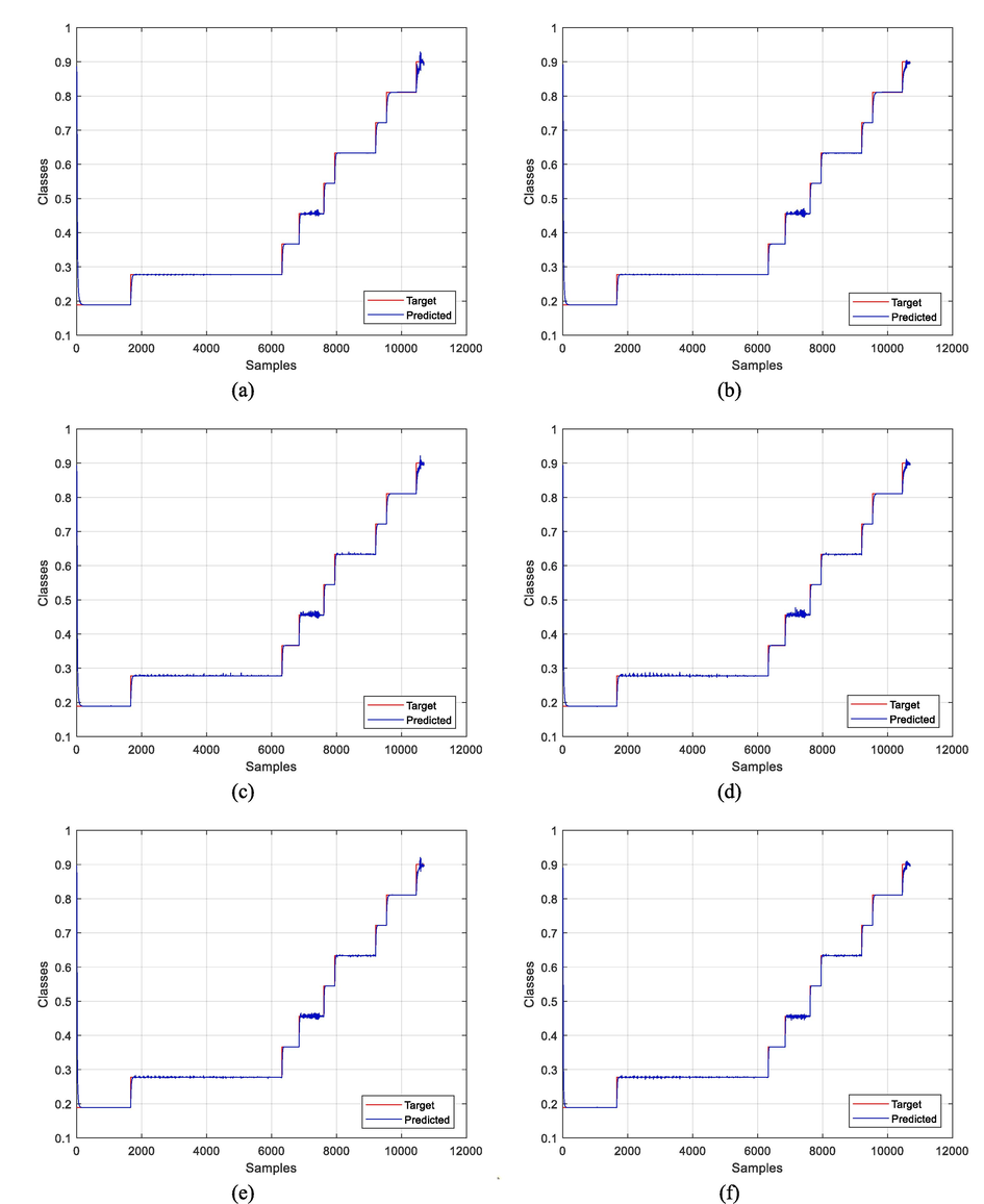
The following Fig. 3 shows the behavior of each experiment conducted on the Indian Pines dataset and the effect of each experiment under some conditions and hyperparameters. Where, we notice some models give better results than others depending on the type of features extracted, as well as their impact on the model during learning. Some models are weak in finding all classes, but we note the best result obtained by BPVAM-PCA with 80 features.
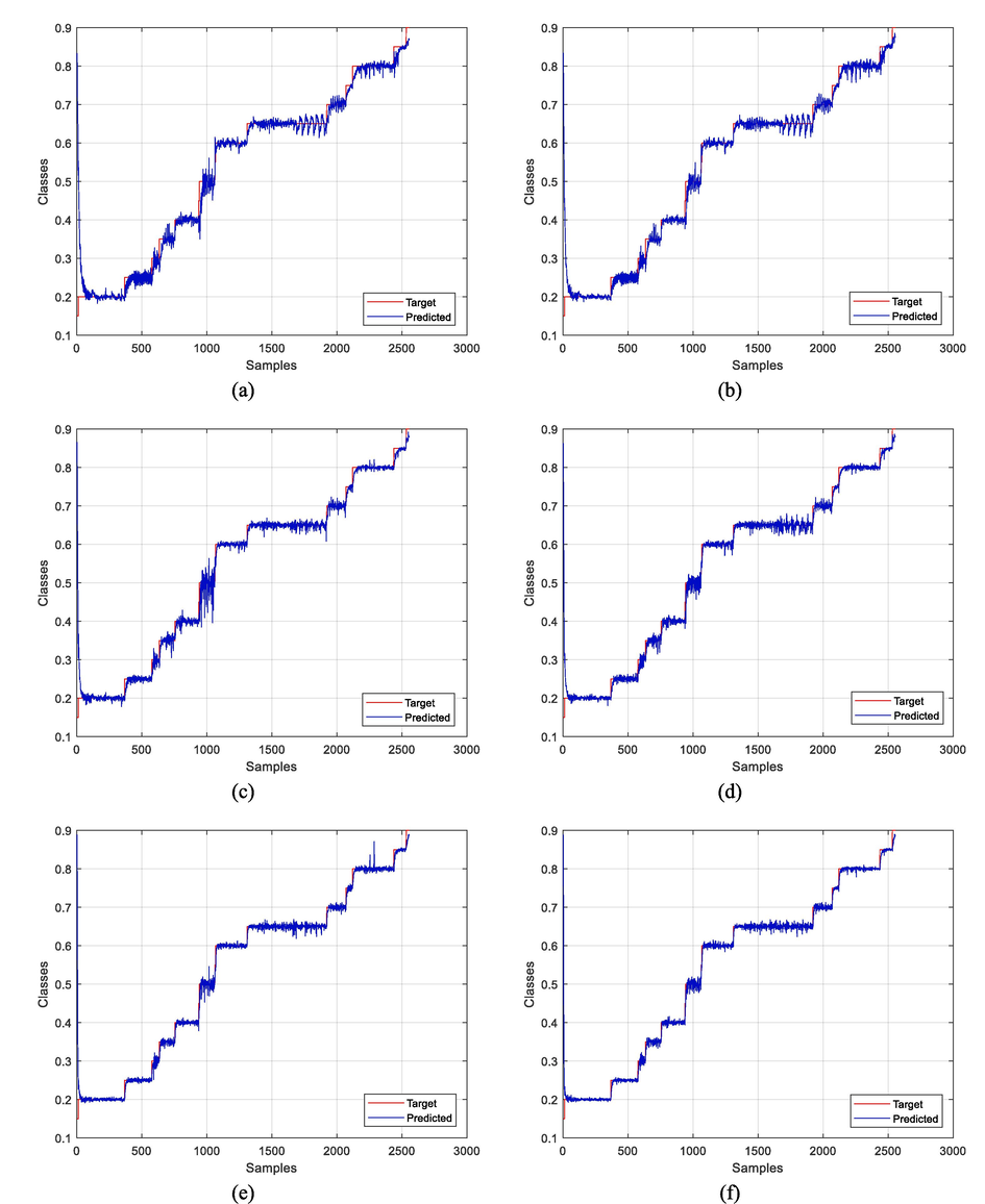
- Predicted classes by BP-PCA and BPVAM-PCA methods using different features for Indian Pines dataset. a) BP-PCA with 10 features. b) BPVAM-PCA with 10 features. c) BP-PCA with 40 features. d) BPVAM-PCA with 40 features. e) BP-PCA with 80 features. f) BPVAM-PCA with 80 features.
4.2 Pavia University dataset
The second experiment is performed using The University of Pavia hyperspectral dataset. Since the number of bands in The University of Pavia dataset was relatively less (103) than the Indian Pines dataset (200), a set of smaller features was selected. Three different combinations were tested for different feature sizes: 5, 10 and 20. As mentioned earlier, these sizes were empirically calculated by running the experiment several times. The dataset was split into training (75 %) and testing (30 %) subsets.
Table 3 summarizes the results obtained for BP-PCA and BPVAM-PCA models for the Pavia University dataset with varying size of features. It is clearly seen from the table that the proposed BPVAM-PCA model outperformed BP-PCA by improving the classification accuracies with all three different feature sizes. BPVAM-PCA for feature size of 20 produced more accurate results with accuracy = 99.71 % and error = 2.16 for training and accuracy = 99.11 % and SSE = 2.15 for testing dataset. Compared with BPVAM, BP-PCA achieved relatively low performance with accuracy = 99.64 % and SSE = 2.73 for training, and accuracy = 98.88 % and SSE = 2.72 for the test datasets. For features size 5, BP-PCA produced the lowest testing accuracy (99.53 %) with high SSE (3.5). In contrast, the performance of BPVAM-PCA was relatively better in terms of accuracy (99.54 %) and SSE (3.2). Similarly, for feature size 10, both models exhibited similar behavior, yet BPVAM-PCA proved to be more accurate for both test and training. This shows that BPVAM-PCA maintains its robustness by iteratively adapting itself using variable momentum, then gives better results than other models when tested with varying sizes of features.
| Feature Size | Method | Training | Testing | ||
|---|---|---|---|---|---|
| Accuracy | SSE | Accuracy | SSE | ||
| 5 | BP-PCA | 99.53 | 3.5268 | 98.48 | 3.5002 |
| BPVAM-PCA | 99.54 | 3.2405 | 98.61 | 3.1362 | |
| 10 | BP-PCA | 99.56 | 3.2101 | 98.62 | 3.2007 |
| BPVAM-PCA | 99.58 | 3.0997 | 98.71 | 3.0923 | |
| 20 | BP-PCA | 99.64 | 2.7325 | 98.88 | 2.7260 |
| BPVAM-PCA | 99.71 | 2.1678 | 99.11 | 2.1586 | |
Table 4 presents Pre, Rec, Spe, and F1 results for two classification methods, BP-PCA and BPVAM-PCA, evaluated across three distinct feature sizes (5, 10, and 20) using the University of Pavia dataset, which comprises nine land cover classes. BPVAM-PCA demonstrates slightly higher precision, recall, and specificity values across most classes and feature sizes, indicating its proficiency in classifying land cover types. The performance comparison between BP-PCA and BPVAM-PCA, as shown in the presented results, reveals that BPVAM-PCA consistently achieves F1-scores close to 1, suggesting a well-balanced trade-off between precision and recall.
| Method | Label | Class | Feature Size (5) | Feature Size (10) | Feature Size (20) | |||||||||
|---|---|---|---|---|---|---|---|---|---|---|---|---|---|---|
| Pre. | Rec. | Spe. | F1 | Pre. | Rec. | Spe. | F1 | Pre. | Rec. | Spe. | F1 | |||
| BP-PCA | 1 | Asphalt | 0.99 | 0.97 | 1.00 | 0.98 | 0.99 | 0.97 | 1.00 | 0.98 | 0.99 | 0.98 | 1.00 | 0.98 |
| 2 | Meadows | 0.99 | 1.00 | 0.99 | 0.99 | 0.99 | 1.00 | 1.00 | 0.99 | 0.99 | 1.00 | 1.00 | 1.00 | |
| 3 | Gravel | 0.97 | 0.98 | 1.00 | 0.97 | 0.97 | 0.98 | 1.00 | 0.98 | 0.98 | 0.98 | 1.00 | 0.98 | |
| 4 | Trees | 0.98 | 0.99 | 1.00 | 0.98 | 0.98 | 0.99 | 1.00 | 0.99 | 0.99 | 0.99 | 1.00 | 0.99 | |
| 5 | Painted metal sheets | 0.96 | 0.97 | 1.00 | 0.97 | 0.97 | 0.98 | 1.00 | 0.97 | 0.97 | 0.98 | 1.00 | 0.98 | |
| 6 | Bare Soil | 0.99 | 0.99 | 1.00 | 0.99 | 0.99 | 0.99 | 1.00 | 0.99 | 0.99 | 0.99 | 1.00 | 0.99 | |
| 7 | Bitumen | 0.94 | 0.97 | 1.00 | 0.96 | 0.95 | 0.97 | 1.00 | 0.96 | 0.96 | 0.98 | 1.00 | 0.97 | |
| 8 | Self-Blocking Bricks | 0.97 | 0.98 | 1.00 | 0.98 | 0.97 | 0.98 | 1.00 | 0.98 | 0.97 | 0.99 | 1.00 | 0.98 | |
| 9 | Shadows | 0.99 | 0.90 | 1.00 | 0.94 | 0.98 | 0.89 | 1.00 | 0.94 | 0.99 | 0.92 | 1.00 | 0.95 | |
| BPVAM-PCA | 1 | Asphalt | 0.99 | 0.97 | 1.00 | 0.98 | 0.99 | 0.97 | 1.00 | 0.98 | 0.99 | 0.98 | 1.00 | 0.99 |
| 2 | Meadows | 0.99 | 1.00 | 0.99 | 0.99 | 0.99 | 1.00 | 1.00 | 1.00 | 1.00 | 1.00 | 1.00 | 1.00 | |
| 3 | Gravel | 0.97 | 0.98 | 1.00 | 0.98 | 0.97 | 0.98 | 1.00 | 0.98 | 0.98 | 0.99 | 1.00 | 0.98 | |
| 4 | Trees | 0.98 | 0.99 | 1.00 | 0.99 | 0.99 | 0.99 | 1.00 | 0.99 | 0.99 | 0.99 | 1.00 | 0.99 | |
| 5 | Painted metal sheets | 0.97 | 0.98 | 1.00 | 0.97 | 0.97 | 0.98 | 1.00 | 0.97 | 0.98 | 0.99 | 1.00 | 0.98 | |
| 6 | Bare Soil | 0.99 | 0.99 | 1.00 | 0.99 | 0.99 | 0.99 | 1.00 | 0.99 | 0.99 | 1.00 | 1.00 | 1.00 | |
| 7 | Bitumen | 0.95 | 0.97 | 1.00 | 0.96 | 0.95 | 0.97 | 1.00 | 0.96 | 0.97 | 0.98 | 1.00 | 0.97 | |
| 8 | Self-Blocking Bricks | 0.97 | 0.98 | 1.00 | 0.98 | 0.97 | 0.99 | 1.00 | 0.98 | 0.98 | 0.99 | 1.00 | 0.98 | |
| 9 | Shadows | 0.98 | 0.90 | 1.00 | 0.94 | 0.98 | 0.90 | 1.00 | 0.94 | 0.99 | 0.93 | 1.00 | 0.96 | |
Fig. 4 shows that the BPVAM-PCA model maintained the best performance in terms of low error and speed of convergence for all three extracted features. This indicates that the variable adaptive momentum provided significant performance enhancement for BPVAM-PCA over BP-PCA. Fig. 5 confirms the results shown in Tables 3, and 4 where the experiment was tested on the University of Pavia dataset in 6 different cases under different conditions and hyperparameters. It is clear that the best result was obtained by BPVAM-PCA with 20 features, where the extracted features and selected hyperparameters have a very large impact on the learning model and can also outperform the weaknesses challenges of other comparable models in finding all classes.
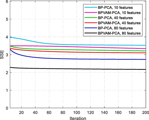
- Convergence behavior of BP-PCA and BPVAM-PCA methods using different features on The University of Pavia dataset.
- Predicted classes by BP-PCA and BPVAM-PCA methods using different features for Pavia University dataset. a) BP-PCA with 5 features. b) BPVAM-PCA with 5 features. c) BP-PCA with 10 features. d) BPVAM-PCA with 10 features. e) BP-PCA with 20 features. f) BPVAM-PCA with 20 features.
When the performance of the two models are compared for both Indian Pines and Pavia University datasets, the best classification results are obtained by the proposed method. In case of the Indian Pines dataset, the feature size of 80 produced the best result, while for the University of Pavia dataset the best performance was obtained for BPVAM-PCA with 20 features. It can be concluded that selecting a few number of features may not be useful as most of the features that carry most significant information are lost. This lead to a suboptimal performance of model in understanding the true patterns of the data. It is worth noting that the dataset had some class imbalance issues, yet the BPVAM-PCA was able to overcome this issue and adapt to learn more about the input patterns with few samples. Generally, when models are trained with imbalance data, their performance may be severely degraded. However, the proposed model's performance remain intact even with imbalance data. This is a highly desirable feature as many multi-class classification problems may have class imbalance issues. Special techniques need to be implemented to deal with it. BPCAM-PCA was able to deal with class imbalance to some extend with ease.
5 Conclusion
This comprehensive study delved into the realm of hyperspectral image classification, focusing on the application of a novel hybrid technique known as BPVAM-PCA. By integrating supervised (Back-Propagation) and unsupervised (Principal Component Analysis) methods, this approach demonstrated significant promise in the field. PCA was initially employed to extract highly discriminant features from hyperspectral images, followed by the application of the BPVAM classifier for pixel-wise classification. The incorporation of a variable adaptive momentum term proved instrumental in enhancing the training speed and overall accuracy of the model. Importantly, the model exhibited a rapid convergence to a steady-error state during the training process, further emphasizing its efficiency in hyperspectral image classification. Comparative analysis with alternative methods, including BP-PCA and BPVAM, on benchmark datasets (Indian Pines and Pavia University) showcased the superiority of the proposed BPVAM-PCA approach. It consistently outperformed its counterparts across various feature sizes and datasets, underscoring its effectiveness in handling the intricacies of hyperspectral image classification.
In the future, the work will be extended to include the exploration of deep feature extraction through convolutional neural networks integrated with the backpropagation model. This promises to eliminate the need for manual feature engineering while further elevating classification accuracy. Additionally, parallel implementations of BPVAM will be explored to leverage GPU capabilities for training models on large-scale datasets. The application of BPVAM in remote sensing, coupled with advancements in smart sensors and IoT, will continue to be a focal point, offering promising prospects in diverse domains, including crop monitoring, environmental assessment, landslide detection, and soil quality evaluation. However, it's important to note that while BPVAM-PCA shows significant promise, potential weaknesses or limitations, such as computational complexity or sensitivity to hyperparameter settings, should also be thoroughly investigated and addressed in future research to ensure its robustness and reliability in real-world applications.
Declaration of competing interest
The authors declare that they have no known competing financial interests or personal relationships that could have appeared to influence the work reported in this paper.
References
- Hybrid convolutional neural network (CNN) for Kennedy Space Center hyperspectral image. Aerospace Syst. 2022:1-8.
- [Google Scholar]
- PulDi-COVID: Chronic obstructive pulmonary (lung) diseases with COVID-19 classification using ensemble deep convolutional neural network from chest X-ray images to minimize severity and mortality rates. Biomed. Signal Process. Control. 2023;81:104445
- [Google Scholar]
- Knowledge distillation: a novel approach for deep feature selection. Egypt. J. Remote Sens. Space Sci.. 2023;26(1):63-73.
- [Google Scholar]
- A novel information gain based approach for classification and dimensionality reduction of hyperspectral images. Procedia Comput. Sci.. 2019;148:126-134.
- [Google Scholar]
- Hybrid 3D/2D complete inception module and convolutional neural network for hyperspectral remote sensing image classification. Neural Process. Lett. 2022:1-44.
- [Google Scholar]
- Spatial-spectral classification of hyperspectral remote sensing images using 3D CNN based LeNet-5 architecture. Infrared Phys. Technol.. 2022;127:104470
- [Google Scholar]
- Machine learning and deep learning techniques for spectral spatial classification of hyperspectral images: a comprehensive survey. Electronics. 2023;12(3):488.
- [Google Scholar]
- Robust adaptive learning approach to self-organizing maps. Knowledge-Based Syst.. 2019;171:25-36.
- [Google Scholar]
- The application of convolutional neural networks for tomographic reconstruction of hyperspectral images. Displays. 2022;74:102218
- [Google Scholar]
- Fuzzy-twin proximal SVM kernel-based deep learning neural network model for hyperspectral image classification. Neural Comput. & Applic.. 2022;34(21):19343-19376.
- [Google Scholar]
- Attention mechanism and depthwise separable convolution aided 3DCNN for hyperspectral remote sensing image classification. Remote Sens. (Basel). 2022;14(9):2215.
- [Google Scholar]
- Internet of Things technology in mineral remote sensing monitoring. Int. J. Circuit Theory Appl.. 2020;48(12):2065-2077.
- [Google Scholar]
- LIII. On lines and planes of closest fit to systems of points in space. London, Edinburgh. Dublin Philos. Mag. J. Sci.. 1901;2:559-572.
- [Google Scholar]
- Study of spatial-spectral feature extraction frameworks with 3-D convolutional neural network for robust hyperspectral imagery classification. IEEE J. Sel. Top. Appl. Earth Obs. Remote Sens.. 2021;14:1717-1727.
- [Google Scholar]
- A multi-temporal method for detection of underground natural gas leakage using hyperspectral imaging. Int. J. Greenh. Gas Control. 2022;117:103659
- [Google Scholar]
- Applications of hyperspectral imaging in plant phenotyping. Trends Plant Sci.. 2022;27:301-315.
- [Google Scholar]
- A deep learning-based intelligent decision support system for hyperspectral image classification using manifold batch structure in Internet of Things (IoT) Wirel. Pers. Commun.. 2022;126(3):2119-2147.
- [Google Scholar]
- Advances in IoT and smart sensors for remote sensing and agriculture applications. Remote Sens. (Basel). 2021;13(13):2585.
- [Google Scholar]
- Application of hyperspectral image anomaly detection algorithm for Internet of things. Multimed. Tools Appl.. 2019;78:5155-5167.
- [Google Scholar]
- Change detection from very-high-spatial-resolution optical remote sensing images: methods, applications, and future directions. IEEE Geosci. Remote Sens. Mag. 2021:2-35.
- [Google Scholar]
- Advances in hyperspectral remote sensing of vegetation traits and functions. Remote Sens. Environ.. 2021;252:112121
- [Google Scholar]
- A combination method of stacked autoencoder and 3D deep residual network for hyperspectral image classification. Int. J. Appl. Earth Obs. Geoinf.. 2021;102:102459
- [Google Scholar]
- A hybrid classification method with dual-channel CNN and KELM for hyperspectral remote sensing images. Int. J. Remote Sens.. 2023;44(1):289-310.
- [Google Scholar]
- Shallow-to-deep spatial-spectral feature enhancement for hyperspectral image classification. Remote Sens. (Basel). 2023;15(1):261.
- [Google Scholar]


