Translate this page into:
Earthquakes magnitude predication using artificial neural network in northern Red Sea area
*Corresponding author. Address: Geology and Geophysics Department, College of Science, King Saud University, Riyadh, Saudi Arabia. Tel.: +966 501005055, fax: +966 14670388. salhumidan@ksu.edu.sa (Saad Al-Humidan)
-
Received: ,
Accepted: ,
This article was originally published by Elsevier and was migrated to Scientific Scholar after the change of Publisher.
Available online 14 May 2011
Peer review under responsibility of King Saud University.
Abstract
Since early ages, people tried to predicate earthquakes using simple observations such as strange or atypical animal behavior. In this paper, we study data collected from past earthquakes to give better forecasting for coming earthquakes. We propose the application of artificial intelligent predication system based on artificial neural network which can be used to predicate the magnitude of future earthquakes in northern Red Sea area including the Sinai Peninsula, the Gulf of Aqaba, and the Gulf of Suez. We present performance evaluation for different configurations and neural network structures that show prediction accuracy compared to other methods. The proposed scheme is built based on feed forward neural network model with multi-hidden layers. The model consists of four phases: data acquisition, pre-processing, feature extraction and neural network training and testing. In this study the neural network model provides higher forecast accuracy than other proposed methods. Neural network model is at least 32% better than other methods. This is due to that neural network is capable to capture non-linear relationship than statistical methods and other proposed methods.
Keywords
Artificial neural network
Back propagation
Multilayer neural network
Artificial intelligent
Earthquake
Prediction system
Northern Red Sea
1 Introduction
Earthquakes are natural hazards that do not happen very often, however they may cause huge losses in life and property. Early preparation for these hazards is a key factor to reduce their damage and consequence. Earthquake forecasting has long attracted the attention of many scientists. In 1975, scientists successful forecasted strong earthquake, Haicheng earthquake, in China using geoelectrical measurements (Wang et al., 2006). Wang et al. (2006) have mentioned that the prediction of Haicheng earthquake was a blend of confusion, empirical analysis, intuitive judgment, and good luck. Despite of that, it was the first successful prediction for a major earthquake. One year later, the scientists failed to predict the Tangshan earthquake, a strong earthquake in the region. This failure of prediction of the Tangshan earthquake caused heavy losses of lives and properties, an estimated 250,000 fatalities and 164,000 injured.
There are several earthquake anomalies that have been used and found to be associated with earthquakes, such as; pattern of occurrences of earthquakes, high occurrences of earthquakes during full/new moon periods, gas and liquid movement before earthquake, change in water and oil levels in wells, electromagnetic anomalies, change in earth gravitational, unusual weather, strange or atypical animal behavior, thermal anomalies, radon anomalies, hydrological anomalies, and abnormal cloud.
QuakeSim is a NASA project for modeling and understanding earthquake and tectonic processes mainly for California state in USA (http://quakesim.jpl.nasa.gov/index.html, July 2009). The main goal of QuakeSim is to develop an accurate earthquakes forecasting to mitigate their danger. QuakeSim team has published their first “Scorecard” which is a forecast map for expected area where major earthquakes (magnitude > 5.0) may happen for the period of time January 1, 2000–December 31, 2009. The scorecard was successful since 25 of the 27 scorecard events occurred after the scorecard was first published on 2002 in the proceedings of the National Academy of Sciences (Rundle et al., 2002).
Paul et al. (1998) estimated the focal parameters of Uttarkashi earthquake using peak ground horizontal accelerations. The observed radiation pattern is compared with the theoretical radiation pattern for different value of focal parameter. Murthy (2002) have studied the spatial distribution of earthquakes and their correlation with geophysical mega lineaments in the Indian subcontinent.
Some Statistical methods are used for long-term earthquake prediction; however it is hard to apply the same statistical methods for short-term earthquake prediction. Anderson (1981) has proposed using Bayesian model to predict earthquake. Varotsos et al. have used seismic electric signals to provide short-term earthquake prediction in Greece (Varotsos and Alexopoulos, 1984a,1984b; Varotsos et al., 1996). Latoussakis and Kossobokov (1990) have applied M8 algorithm to provide intermediate-term earthquake prediction in Greece. The M8 algorithm makes intermediate term predictions for earthquakes to occur in a large circle, based on integral counts of transient seismicity in the circle. Varotsos et al. (1988, 1989) have proposed VAN method which is an experimental method of earthquake prediction. The VAN method is named after the surname initials of its inventors. It is based on observing and assessing seismic electric signals (SES) that occur several hours to days before the earthquake which can be used as warning signs.
Wang et al. (2001) have used single multi-layer perception neural networks to give an estimation of the earthquakes in Chinese Mainland. Panakkat and Adeli have studied neural network models for predicting the magnitude of large earthquake using eight seismicity indicators. The indicators are selected based on Gutenberg-Richter, earthquake magnitude distribution, and recent studies for earthquake prediction. Since there is no known relationship between these indicators and the location and magnitude of a next expected (succeeding) earthquake, three different neural networks are used. The authors have used a feed-forward Levenberg–Marquardt back propagation (LMBP) neural network, a recurrent neural network, and a radial basis function (RBF) neural network.
Bose and Wenzel have developed an earthquake early warning system – called PreSEIS – for finite faults based on neural network (Bose et al., 2008). PreSEIS uses two layer feedforward neural network to estimate the most likely source parameters such as the earthquake hypocenter location, magnitude, and the expansion of evolving seismic rupture. PreSEIS rely on the available information on ground motions at different sensors in a seismic network to provide better estimation.
Kulachi et al. (2009) model the relationship between radon and earthquake using a three-layer artificial neural networks with Levenberg–Marquardt learning. They have studied eight different parameters during earthquake occurrence in the East Anatolian Fault System (EAFS).
Despite the importance of earthquake forecasting, it is still a challenge problem for several reasons. The complexity of earthquake forecast has driven the scientists to apply increasingly sophisticated methodologies to simulate earthquake processes. The complexity can be summarized as follows:
-
The earthquake process model is not complete yet, since there are unknown factors that may play roles in existence of new earthquakes.
-
Even for well-known factors, some of them are hard or impossible to measure.
-
The relationship between these factors and the existence of new earthquake is a non-linear (not simple) relationship.
The contributions of our paper are summarized in the following:
-
We propose a new neural network model to predict earthquakes in northern Red Sea area. Although there are similar models that have been published before in different areas, to our best knowledge this is the first neural network model to predict earthquake in northern Red Sea area.
-
We analyze the historical earthquakes data in northern Red Sea area for different statistics parameters such as correlation, mean, standard deviation, and other.
-
We present different heuristic prediction methods and we compare their results with our neural network model.
-
Details performance analysis of the proposed forecasting methods shows that the neural network model provides higher forecasting accuracy.
2 Related work
In this section, we show related work for our research paper. We divide this section into two subsections; where the first subsection presents some research papers about earthquake forecasting while the second subsection gives a brief overview about artificial neural network.
2.1 Earthquake forecasting
Su and Zhu (2009) have studied the relationship between the maximum of earthquake affecting coefficient and site and basement condition. They have proposed a model based on artificial neural network. Itai et al. (2005) have proposed a multilayer using compression data for precursor signal detection in electromagnetic wave observation. Plagianakos and Tzanaki (2001) have applied chaotic analysis approach to a time series composed of seismic events occurred in Greece. After chaotic analysis, an artificial neural network was used to provide short term forecasting. Panakkat and Adeli (2007) have presented new neural network models for large earthquake magnitude prediction in the following month using eight mathematically computed parameters known as seismicity indicators. Lakshmi and Tiwari (2009) have studied a non-linear forecasting technique and artificial neural network methods to model dissection from earthquake time series. They have utilized these methods to characterize model behavior of earthquake dynamics in northeast India. Kulachi et al. (2009) have studied the relationship between radon and earthquake using an artificial neural networks model. Panakkat and Adeli (2009) have proposed a new recurrent neural network model to predict earthquake time and location using a vector of eight seismicity indicators as input.
Negarestani et al. (2002) have proposed layered neural networks to analysis the relationship between radon concentration and environmental parameters in earthquake prediction in Thailand which can give a better estimation of radon variations. Ozerdem et al. (2006) have studied the spatio-temporal electric field data measured by different stations and the regional seismicity. They have proposed neural network for classification and provide an accurate earthquake prediction. Ni et al. (2006) have used PCA-compressed frequency response functions and neural networks to investigate seismic damage identification.
Zhihuan and Junjing (1990) have considered earthquake damage prediction as fuzzy-random event. Jusoh et al. (2008) have investigated the existence of the ionospheric Total Electron Content (TEC) using GPS dual frequency data. The variation of TEC can be considered as an anomaly a few days or hours before the earthquake. Shimizu et al. (2008) have proposed using recursive sample-entropy technique for earthquake forecasting, where they have used the earth data based on VAN method. Turmov et al. (2000) have presented models of predication for earthquakes and tsunami based on simultaneous measurement of elastic and electromagnetic waves.
2.2 Overview of artificial neural network
Artificial neural network, usually called neural network, is a mathematical model that simulates the structure and functionality of biological neural networks. Neural network is a network of nodes – also called neuron – connected by directed links, where every linki,j that connects nodei to nodej has a numeric weight wi,j associated with it, also there is an activation function f associate with every nodej. The weight determines how much the input contributes to and affects the result of the activation function. The activation function will be applied to the sum of inputs multiple by the weights for all incoming links, as shown in Fig. 1. Any weight is called a bias weight whenever its input is a fixed value of −1, which can be used to shift the activation function regardless of the inputs.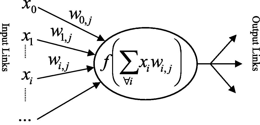
A simple mathematical model for a neuron.
The activation function – also called transfer function – defines the output of that node given an input or set of inputs. The activation function needs to be nonlinear, otherwise the entire neural network becomes a simple linear function. Nonlinear activation function allows the neural network to deal with nontrivial problems using a small number of nodes. Neural Networks support a wide range of activation functions such as; step function, linear function, sign function, and sigmoid function, as shown in Fig. 2. The sigmoid function is considered the most popular activation function mainly for two reasons – firstly, it is differentiable so it possible to derive a gradient search learning algorithm for networks with multiple layers, and secondly, it is continuous-valued output rather than binary output produced by the hard-limiter.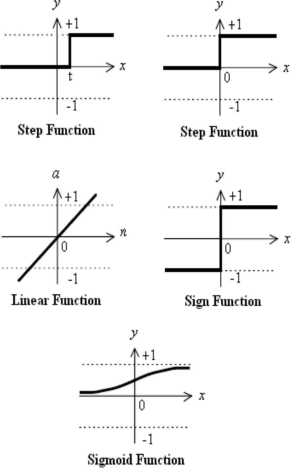
Some common activation functions.
There are two main types of neural network structures; feedforward networks and recurrent networks. A feedforward network is acyclic network so it has no internal state other than the weights themselves. In the other side, a recurrent network is a cyclic network so the network has a state since the outputs are feeded back into the network. As result of that, recurrent networks support short-term memory unlike feedforward networks.
Feedforward networks are usually arranged in layers, where each neuron receives inputs only from the immediately preceding layer. Feedforward networks can be classified into: single layer feedforward neural networks – also called perceptron – and multilayer feedforward neural networks.
For perceptron, all the inputs connected directly to the output neurons and there is no hidden layer. In this manner, every weight affects only one output neuron. When there is a single output neuron, the network is called single perceptron, as shown in Fig. 3.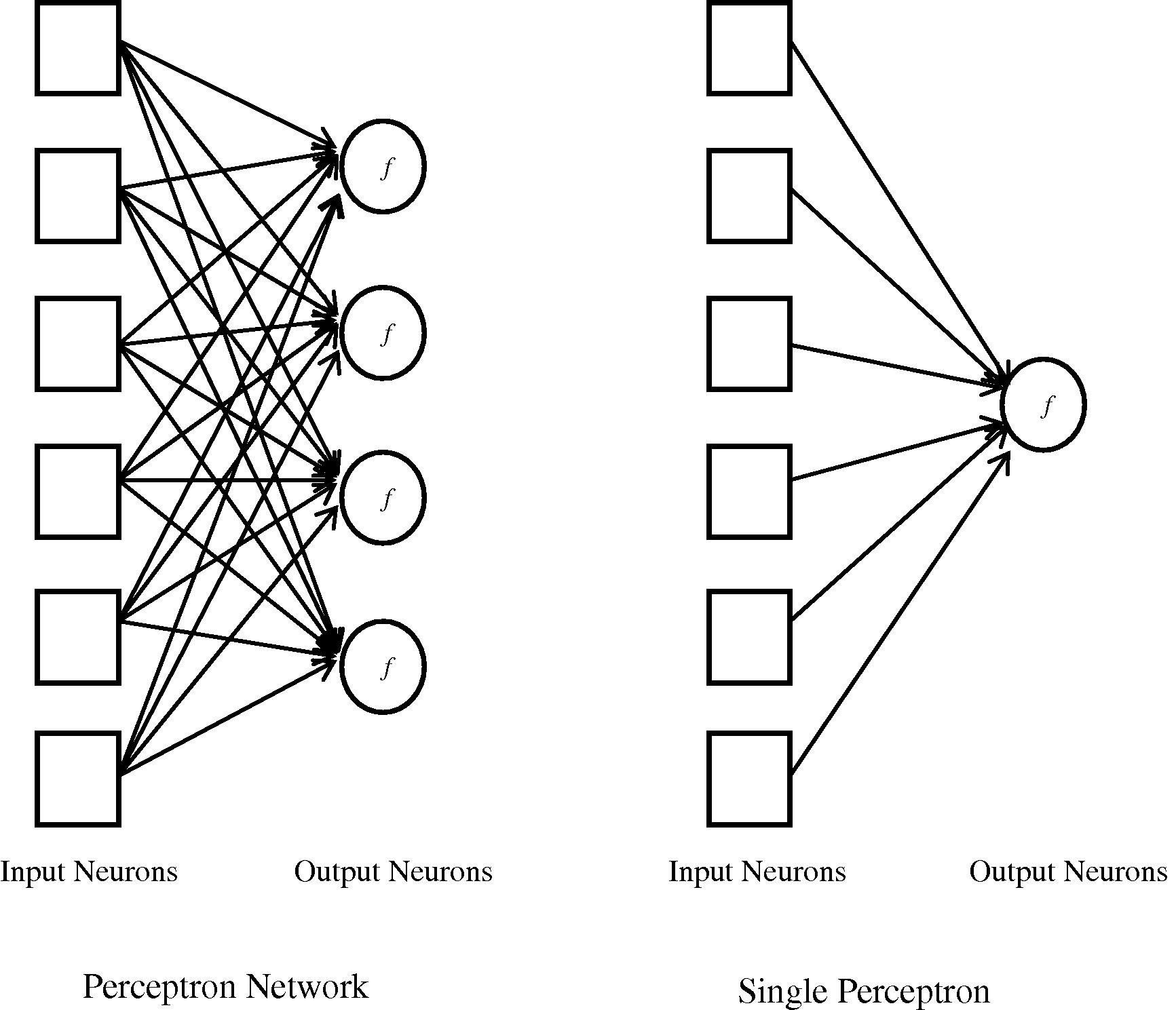
Shows the design of the neural network.
Perceptron is able to represent any linear separable function such as AND, OR, and NOT Boolean functions and majority function. On the other hand, perceptron is not able to represent XOR Boolean function since XOR is not linear separable. Despite perceptron limitations, perceptron has a simple learning algorithm that will fit the perceptron to any linearly separable function.
Hidden layers feed forward neural network – sometimes called backpropagation network – can be used to solve non-linear problems such XOR and many more difficult problems. Hidden layer feedforward neural network currently accounts for 80% of all neural network applications. A simple version of hidden layer feedforward neural network is when a single hidden layer is added and the discrete activation function is replaced with a nonlinear continuous one, as shown in Fig. 4.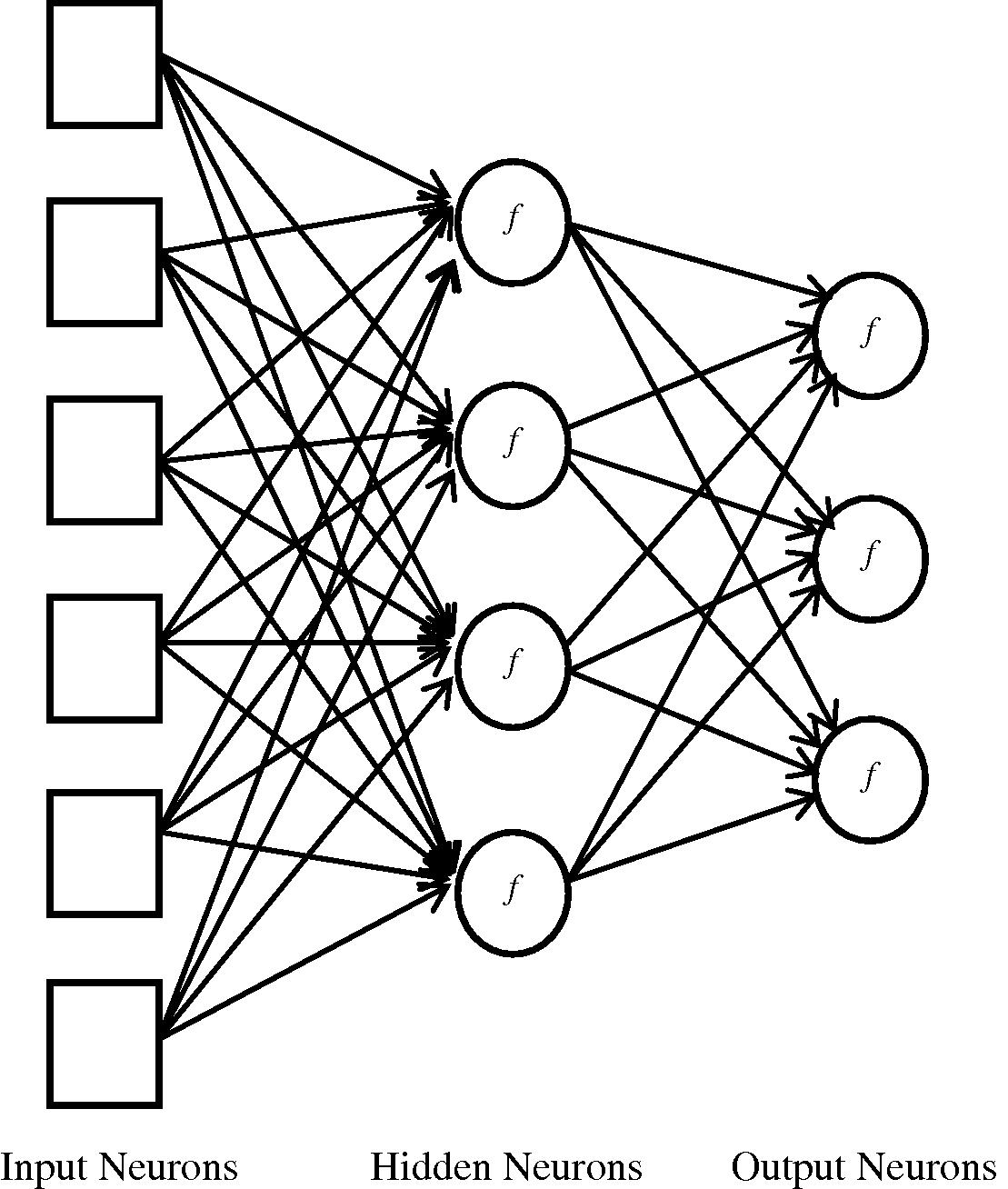
A 3-layer (single hidden layer) feedforward neural network.
The biggest challenge in this type of network was the problem of how to adjust the weights from input to hidden units. Rumelhart et al. (1986) have proposed back propagation learning algorithm, where the errors for the neurons of the hidden layer are determined by back-propagating the errors of the neurons of the output layer.
There are many applications for neural networks such as marketing tactician, computer games, data compression, driving guidance, noise filtering, financial prediction, hand-written character recognition, pattern recognition, computer vision, speech recognition, words processing, aerospace systems, credit card activity monitoring, insurance policy application evaluation, oil and gas exploration, and robotics.
3 The study area
Sinai subplate at the northern Red Sea area occurs between two big plates; African plate and Arabian plate. The plate movement causes the Arabian Peninsula to move northeast which yields the opening of the Red Sea which puts a huge stress along the Aqaba area. This explains transform fault system in the area. Most Moderate and large earthquakes in northern Red Sea area occurred at the boundaries of the Sinai sub-plate such as; Dead Sea Fault System in the east, and Suez rift in the southwest. In fact, most earthquakes events concentrate at the southern and central segments of the Dead Sea Fault System. In the last two decades, there were three swarms (February, 1983; April, 1990; August, 1993 and November, 1995) in the Gulf of Aqaba (southern segment of the Dead Sea Fault System). The Gulf of Aqaba experienced the largest earthquake in the area with moment magnitude (Mw) 7.2 in 1995. A detail statistical analysis for northern Red Sea area is presented in the next section.
During the last century, most events have small magnitudes. There were only two major events that have been recorded in the northern Red Sea area and the neighboring area. The first major event occurred in July 11th, 1927, when an earthquake struck Palestine and killed around 342. Its magnitude was 6.25 and epicentered some 25 km north of the Dead Sea. The second major event occurred in November 22, 1995, when the largest earthquake with magnitude 7.2 struck the Gulf of Aqaba and its aftershocks continued until December 25, 1998. The earthquake was felt over a wide area such as Lebanon, southern Syria, western Iraq, northern Saudi Arabia, Egypt and northern Sudan. The main damages were in Aqaba area such as Elat, Haql and Nuweiba. The earthquake killed at least 11 people and injured 47.
Although the area recorded two major earthquakes during the last century, it suffered from four earthquakes swarms. The first swarm occurred in the Gulf of Aqaba area on January 21, 1983 and lasted for a few months. The second swarm occurred in the Gulf of Aqaba area too on April 20, 1990 and lasted for a week. The third swarm started on July 31, 1993, and continued until the end of August of that year. The fourth swarm was on November 22, 1995, which continued until December 25, 1998.
Historical earthquakes in the area were reported and documented. A major earthquake struck on the morning of March 18th 1068 AD and killed nearly 20,000 people. The earthquake completely destroyed Aqaba and Elat cities. More than a hundred years later, another major earthquake struck the area in 1212 AD. Based on reported damages, a magnitude of at least 7 was derived. There were many reports about damages in nearby area such as western of Jordon where Karak towers were destroyed. Another major earthquake was reported on 1293 AD which struck Gaza region.
4 Data analysis
In this section, we present statistical analysis of the data that we acquired using earthquakes catalog. Statistical analysis is an efficient way of collecting information from a large pool of data. We present the values of several statistical parameters such as mean, mean absolute deviation, median, mode, standard deviation, sample variance, kurtosis, skewness, range, minimum, maximum, sum, count over the earthquakes events including date (year, month, and day), locations (latitude and longitude), and magnitude, as shown in Table 1. These values are to provide the reader with the sense about values distribution which improves our decision-making. They also can be used to judge and evaluate any forecasting methods for northern Red Sea area.
Statistical parameter
Year
Month
Day
Latitude
Longitude
Magnitude
Mean
1994.8
6.7383
14.0062
29.0922
34.6462
3.8798
Mean absolute deviation
2.2799
3.9852
8.5115
0.5009
0.3904
0.6777
Median
1995
8
12
28.9
34.7
4
Mode
1995
12
3
28.5
34.7
4
Standard deviation
4.0994
4.3316
9.5253
0.7664
0.6531
0.8542
Sample variance
16.8049
18.7626
90.7312
0.5874
0.4265
0.7297
Kurtosis
10.7431
1.3564
1.6029
7.5874
7.576
3.1386
Skewness
−0.443
−0.1351
0.2143
2.1958
−1.9616
−0.2798
Range
39
11
30
3.992
3.9
5.3
Minimum
1969
1
1
28
32
1.9
Maximum
2008
12
31
32
35.9
7.2
Sum
640340
2160
4500
9340
11120
1250
Count
321
321
321
321
321
321
Skewness and kurtosis show that the earthquakes events do not carry any symmetry. The mean and median for locations (latitudes and longitudes) show the center where most earthquakes events occurred and concentrated, while the standard deviation shows dispersion level of the data. For these values, we notice that most of earthquakes events concentrated at the Gulf of Aqaba. Although that data were collected for the events between 1969 and 2008, almost 65% of the events located between 1990 and 1998. The table also provides statistical analysis for magnitude values that we are looking to predict which show their range, concentration, dispersion and others (Fig. 5).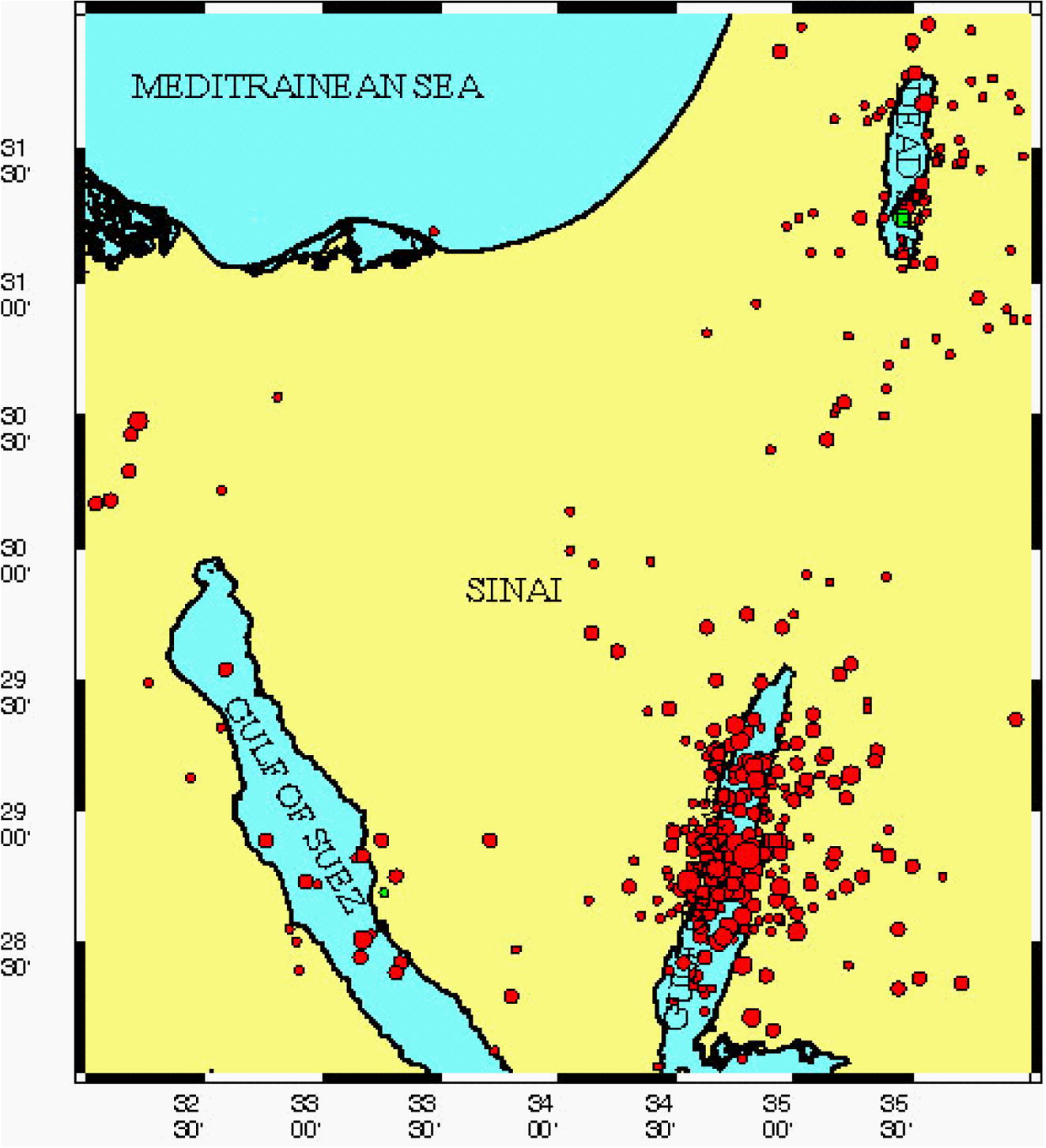
Seismic activities map for Northern Red Sea area from 1969 to 2009.
Beside Table 1, we present several figures which provide a deep analysis for our data. Fig. 6 shows the earthquakes magnitude on time sequence axis, so instead of considering date and time we used sequence numbers. On the other hand, Fig. 7 uses date and time to plot earthquakes magnitude. The yearly earthquakes magnitude range which is the deference between maximum and minimum magnitude for each year is shown in Fig. 8. The magnitude range increases between 1993 and 1996. The distribution of earthquakes events over the years is shown in Fig. 9, which shows that almost 30% of the earthquakes occurred in 1995 and the majority of events occurred between 1992 and 1996.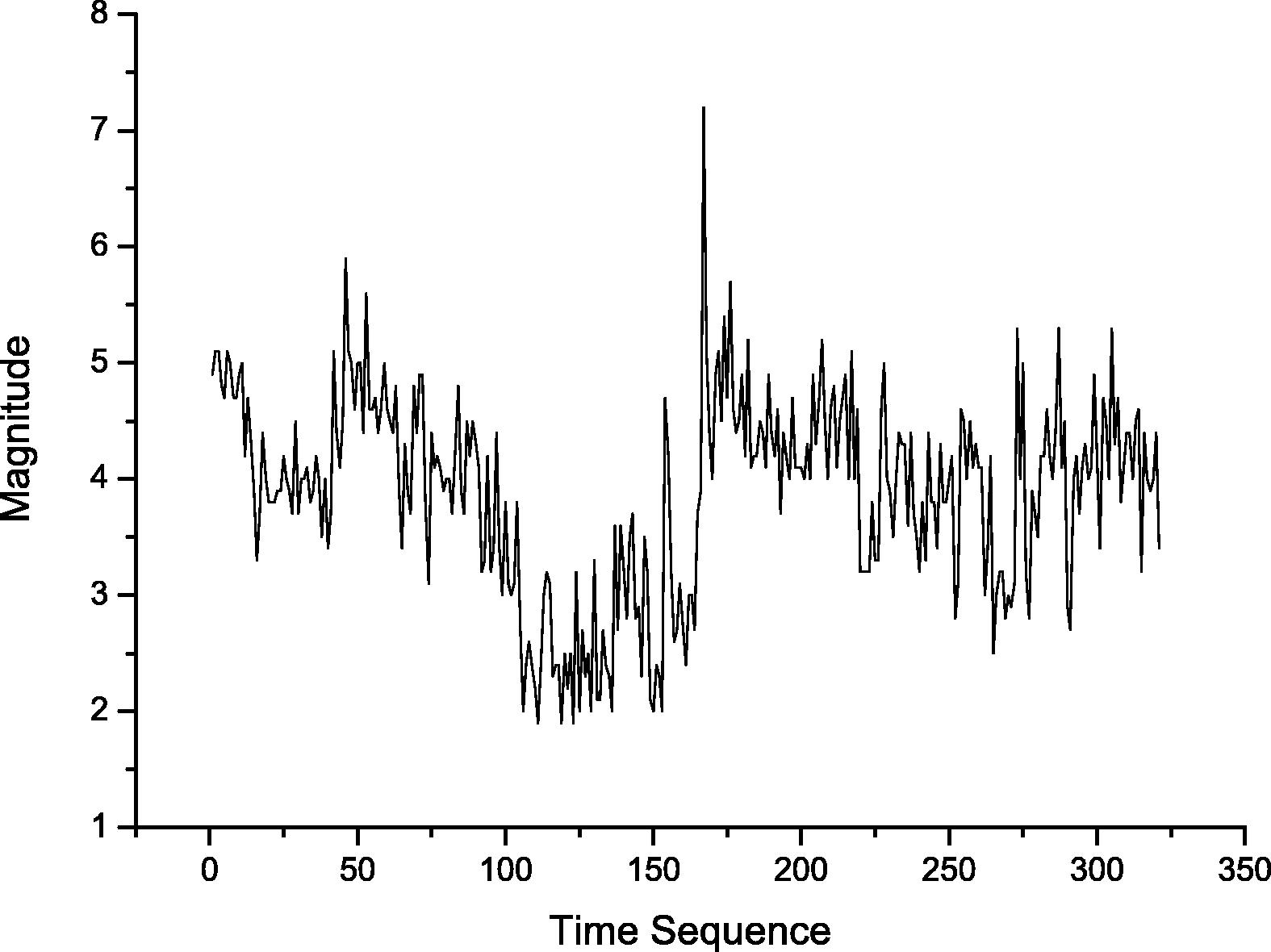
Earthquakes magnitude on time sequence axis.
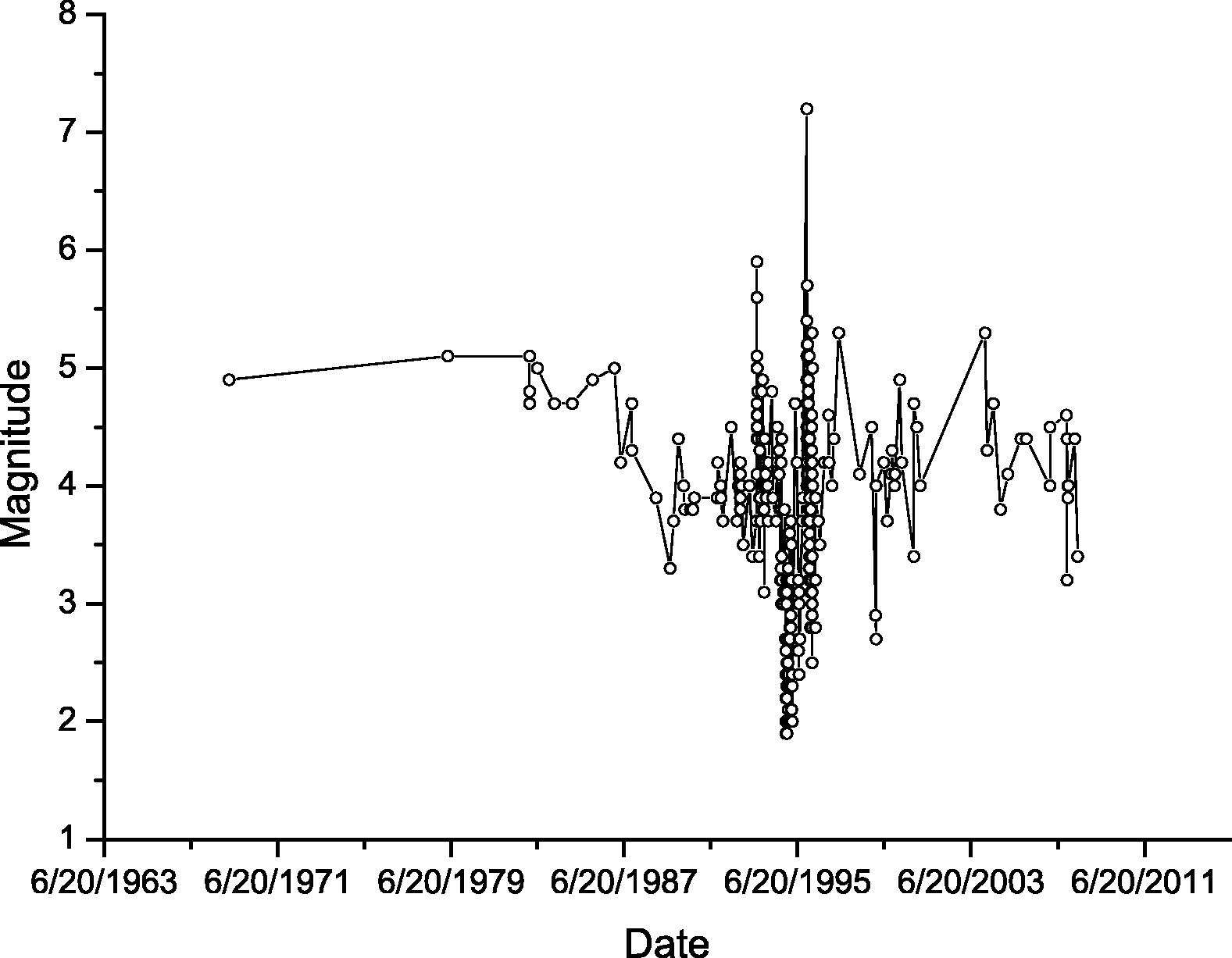
Earthquakes magnitude on date and time axis.
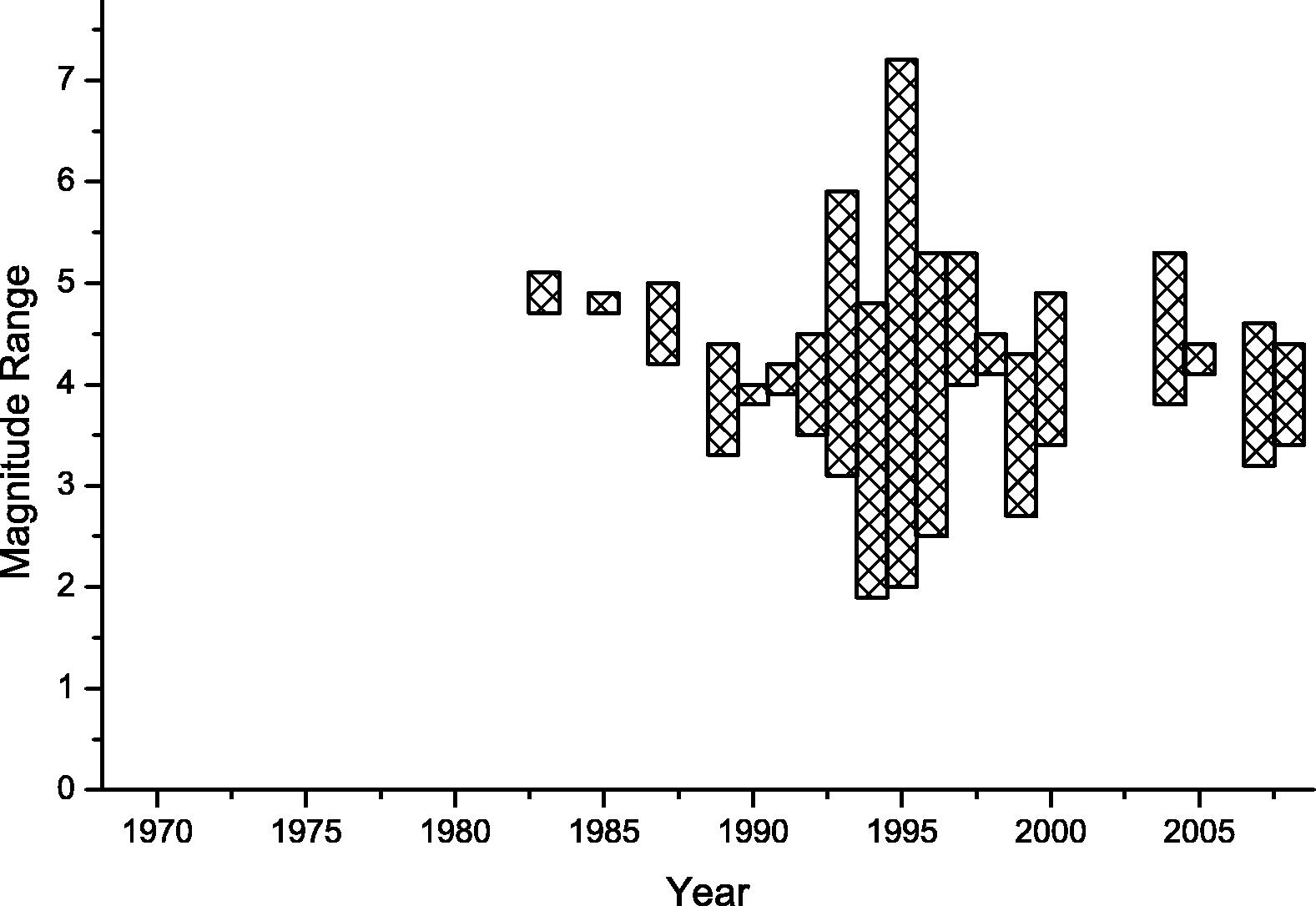
Earthquakes magnitude range (difference between maximum and minimum magnitude) from 1969 to 2009.
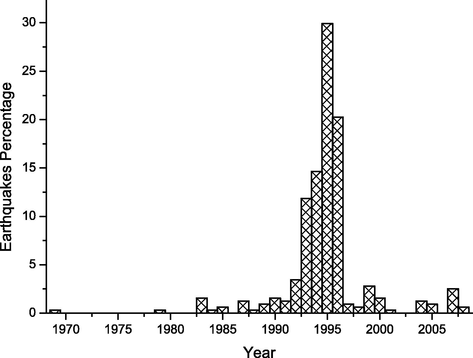
Earthquakes percentage per year from 1969 to 2009.
The histogram of earthquakes events over the year is shown in Fig. 10. The figure shows that most (52% of the events) occurred in January, February and December. This occurred because – as we have shown before – most of the earthquakes occurred on 1994 and 1995, where most of these earthquakes occurred during January, February and December. Another histogram is shown in Fig. 11, which show earthquakes distribution per hour. The figure shows that the distribution is almost uniform distribution which shows no pattern there. It also shows that the time may not add any significant value for any forecasting methods in northern Red Sea area including our neural network model of predication.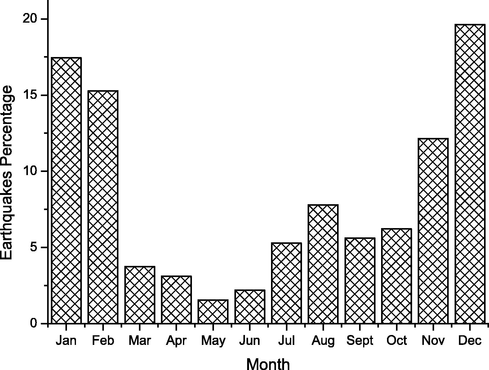
Earthquakes percentage per month.
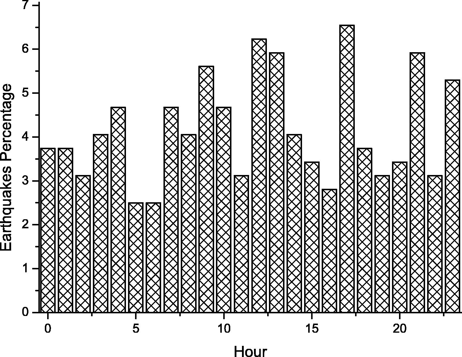
Earthquakes percentage per hour.
In response to a few claims about the relationship between earthquakes and moon phase, we present a bar chart for earthquakes percentage for different magnitude over the moon phases as shown in Fig. 12. The figure shows no significant relationship between moon phase and earthquake except a slight increase in earthquakes percentage of magnitude between 4 and 6 when the phase is close to full moon.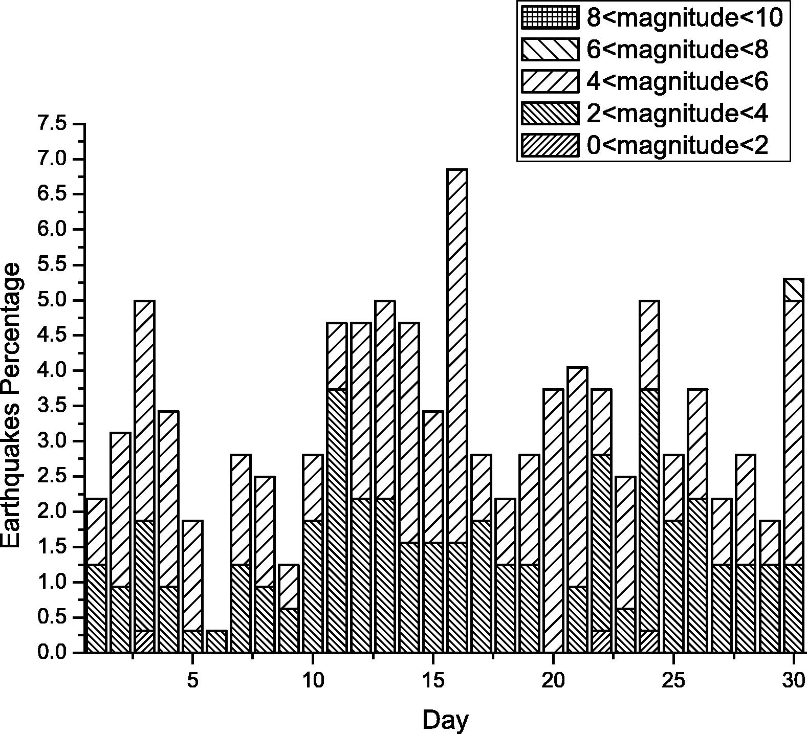
Earthquakes percentage for different magnitude during moon phases.
Fig. 13 shows a histogram of earthquake percentage over different source depths which is almost 85% of earthquakes occurred at depth between 6 km and 10 km. We can conclude for this figure that the source depth may not help in predicting future earthquakes since most of them concentrate within a short range between 6 km and 10 km. Another histogram for earthquakes percentage over different magnitude range is shown in figure. The distribution of the data in this histogram is nearly normal distribution. This figure and statistical value of magnitude in Table 1 can be used to provide indication of how good any magnitude prediction method is (Fig. 14).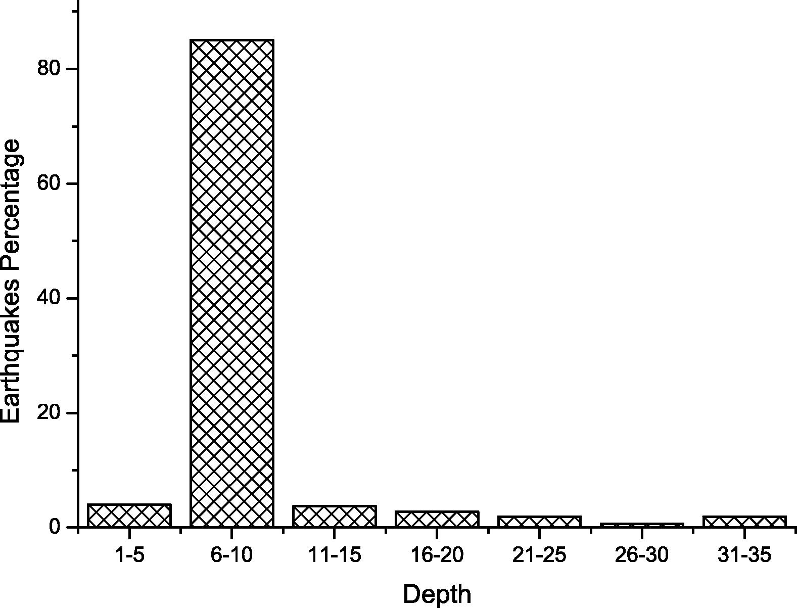
Earthquakes percentage for different source depth.
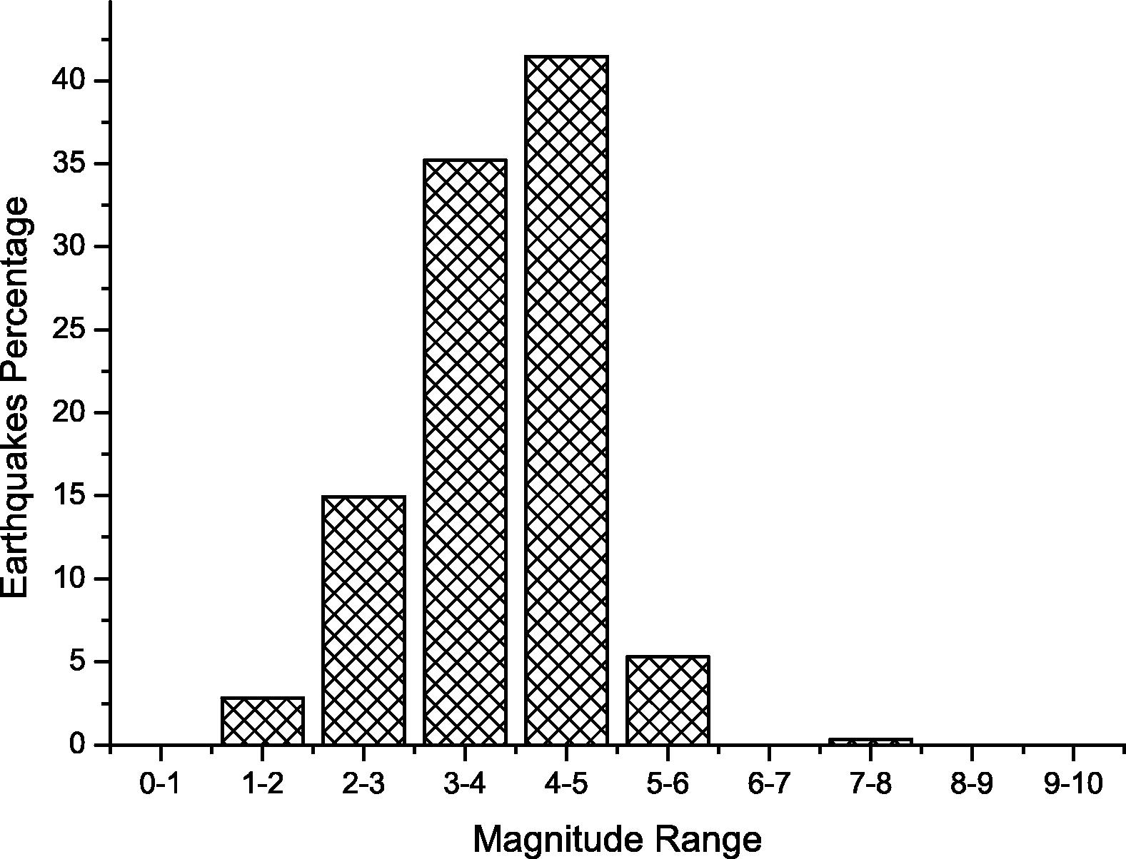
Earthquakes percentage classified based on their magnitude.
5 Mythology
The proposed model is built based on feed forward neural network model with multi-hidden layers to provide earthquake magnitude prediction with high accuracy. In this section, we describe the components of the proposed neural network model. We focus now on the design of the model. As we mentioned before, the model consists of four phases: data acquisition, preprocessing, feature extraction and neural network training and testing as shown in Fig. 15.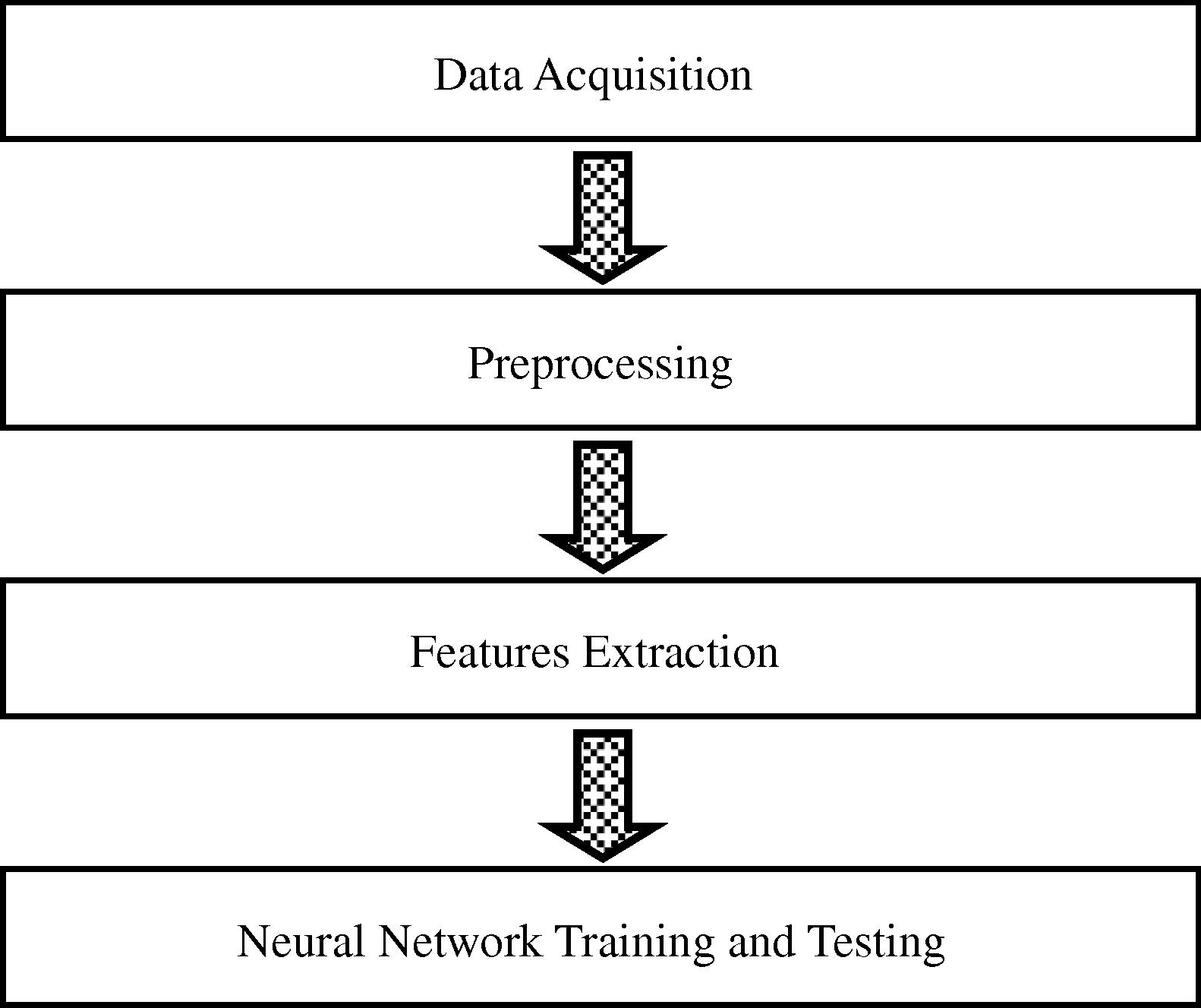
The four main phases of our neural network model.
The proposed scheme consists of four major steps: First, data is acquired from reliable source or multiple sources. This step is very crucial for any forecasting system since poor inputs will generate low-accuracy or invalid outputs.
Second, the historical data is pre-processed and reformatted to be compatible with next phases. One of the main purposes of the pre-processing phase is to eliminate as much noise as possible and to reduce data variation. Also, the pure historical data may not be suitable for use directly either because it has too much information and details that may drive the proposed forecasting system away from the intended goal; or the critical information are hidden and need to be cleared for extraction.
Third, features should be extracted so they will be used in the fourth step. Feature extraction is a very crucial component of the system. We spent a lot of time optimizing the subset of features to be used. Feature extraction is one of the most difficult and important problems of machine learning and pattern recognition. The selected set of features should be small, whose values efficiently help in the prediction.
Fourth, neural network is constructed, trained and tested. This step is the main one in which machine learning is done and future earthquake magnitude is predicted. We have used different feed forward neural network configuration multi-hidden layers to train and test the proposed model.
5.1 Data acquisition
For any prediction model, the data should be collected from reliable single or multiple sources. There are many public and private organizations which provide earthquake catalog and database for earthquakes over the world. Most of these sources are available over the Internet and provide advance search capabilities such as Advanced National Seismic System (ANSS), National Earthquake Information Center (NEIC), the Northern California Earthquake Data Center (NCEDC), and others. We have gotten the data from the Northern California Earthquake Data Center (NCEDC) where we limit search area with latitude between 28 and 32 and longitude between 32 and 36. Also we have limited collected data for every seismic event to the following; year, month, day, time, latitude, longitude, magnitude, depth. Although, earthquake catalog may provide more information about each seismic event, we believe that other information is irrelative to our prediction model and target. Furthermore, the process of building neural network model is time consuming since there are a large number of network configurations that need to be trained and tested. Without limiting our domain by classifying the data into relative and irrelative, the process of building our system will not be achievable within a reasonable time.
5.2 Preprocessing
After data acquisition, the data should be preprocessed which is mainly filtering first and then reformatting. Filtering is necessary to remove noisy and meaningless data. It also removes each seismic event in case part of its data is missing. However, if the missing part will not be used in some network configurations, the event will not be excluded for these configurations only. In other word, filtering criterions rely on the required data of network configurations for the next two phases. Even after filtering, the data may not be suitable for use directly either because; it has too much information and details that may drive our forecasting system away from the intended goal, or the critical information is hidden and needs to be cleared for features extraction. In order to deal with these two issues, reformatting is necessary to make the data ready for the next phase. For example, the latitude and longitude format is not suitable for the next phase because they provide a high degree of accuracy for the location – 100 × 100 units for each latitude or longitude – which is not necessary. In fact, it complicates the training process and drives the neural network to focus on these small details rather than magnitude prediction. In order to avoid that, we divide area of interest into 16 × 16 tiles. The latitude and longitude are replaced by the tile location. This reduces the number of possibilities by a ratio of 99.84%.
5.3 Features extraction
Feature Extraction is an important process which maps the original features of an event into fewer features which include the main information of the data structure. Feature extraction is used when the input data is too large to be processed or the input data have redundancy. In this manner, feature extraction is a special form of dimensionality reduction and redundancy removal. Features extracted are carefully chosen to allow the relevant information in order to perform the desired task.
We have identified a list of candidate features which can be tested in the next phase to eliminate poor quality sets and determine the best candidates. The features are the following:
-
Earthquake sequence number: This is used to keep reserving the order of earthquake events in our study area. It will be used instead of the year, month, day, and time for reasons. First, the date and time is more complex data type for our neural network model than using the sequence number. Second, our focus is to predict the magnitude of the next earthquake rather than the time of the earthquake which means keeping the date and time is not necessary and the sequence number is sufficient for our target. Third, although the date and time logically may help to provide more accurate prediction, we found out after many experiments the sequence is easier to learn for the neural network configuration that we propose.
-
Tile location: This feature identifies the location in which the earthquake events occurred. As we mentioned earlier, we divide the study area into 16 × 16 tiles instead of latitudes and longitudes. In this manner, each tile is represented by two numbers with a range of value between 0 and 15.
-
Earthquake Magnitude: The main feature which should be considered since it represents the fluctuation of the magnitude.
-
The source Depth: The source depth can be considered as a feature however relationship between this feature and the target magnitude (predicted magnitude) will be studied during the next phase.
It is very important to notice that, we study this feature over a predetermine set of neural network configuration. Based on the training and testing result we cancel some of these features and keep the other. This does not mean the selected features are the best ever for any neural network model.
5.4 Neural network training and testing
In this phase, neural network is constructed with a different set of configurations, then trained, and tested. We have used different feed forward neural network configuration with multi-hidden layers for training and testing. We consider the following parameters during neural network configuration and construction:
-
Hidden layer: We have trained and tested feed forward neural network with one hidden layer, two hidden layers, and three hidden layers.
-
Transfer function: Since we used Neural Network Toolbox 6 edition for Matlab 2008b as training and testing software tool, we have considered three Matlab transfer functions which are Logsig, Tansig, and Purelin.
-
Delay of input data: The delay is the number of consecutive earthquakes that are entered to the neural network together as single input row. We are doing like this because feed forward neural network deals with each input row as a single entity. As a result of that neural network does not draw any relationship between different rows, so we enter multiple consecutive events together to allow feed forward neural network to figure out existing relationship between the events in each input row separately. We have considered different delay value from 0 to 10.
6 Performance evaluation
This section is organized into three subsections. In the first one, we introduce other forecasting methods that will be used as benchmarks and compared them with our neural network model. After that, we present performance metrics that are used to compare between different methods and evaluate them. The performance metrics are selected based on the nature of the problem and the expected needs. They are also selected to measure accurately the performance of the proposed methods. The performance results of our neural network model and other forecasting methods are present in the last subsection. The results are presented to make it easy to compare between the methods and make decisions.
6.1 Benchmarks
As we mentioned before, to our best knowledge our prediction model is the first prediction model in the northern Red Sea area. Due to that, we need to compare the performance of our model with other methods that we propose too.
-
Normal distributed random predictor: assuming that earthquakes magnitude distribution is normal, we used the normal distributed random predictor to generate random normal magnitude distribution on and we tested this method with different standard deviation, then we fixed the mean magnitude value (Fig. 16).
-
Uniformly distributed random predictor: This method is similar to normally distributed random predictor however it follows uniform distribution. We also evaluated this method using different range value (difference between maximum and minimum possible value) as shown in Fig. 17.
-
Moving average predictor: Moving average is used to analyze a series of values by creating a series of averages of different subsets of these values. A moving average may also use unequal weights for each value in the series to emphasize particular values. A moving average is commonly used with time series data to determine trends or cycles, for example in technical analysis of financial data. We have used a simple moving average which is the unweighted moving average. The simple moving average of period n is define as following:
-
We have evaluated this method over the earthquake events as shown in Fig. 18 and Table 2.
-
Curve fitting methods: In which several statistical methods for curve fitting are used such as linear regression, quadratic regression, cubic regression, and 4th to 6th degree regression. In all these methods, we try to construct a curve, or mathematical function, that has the best fit to the series of earthquakes magnitudes in the northern Red Sea area. The performance of these methods is shown in Table 2.
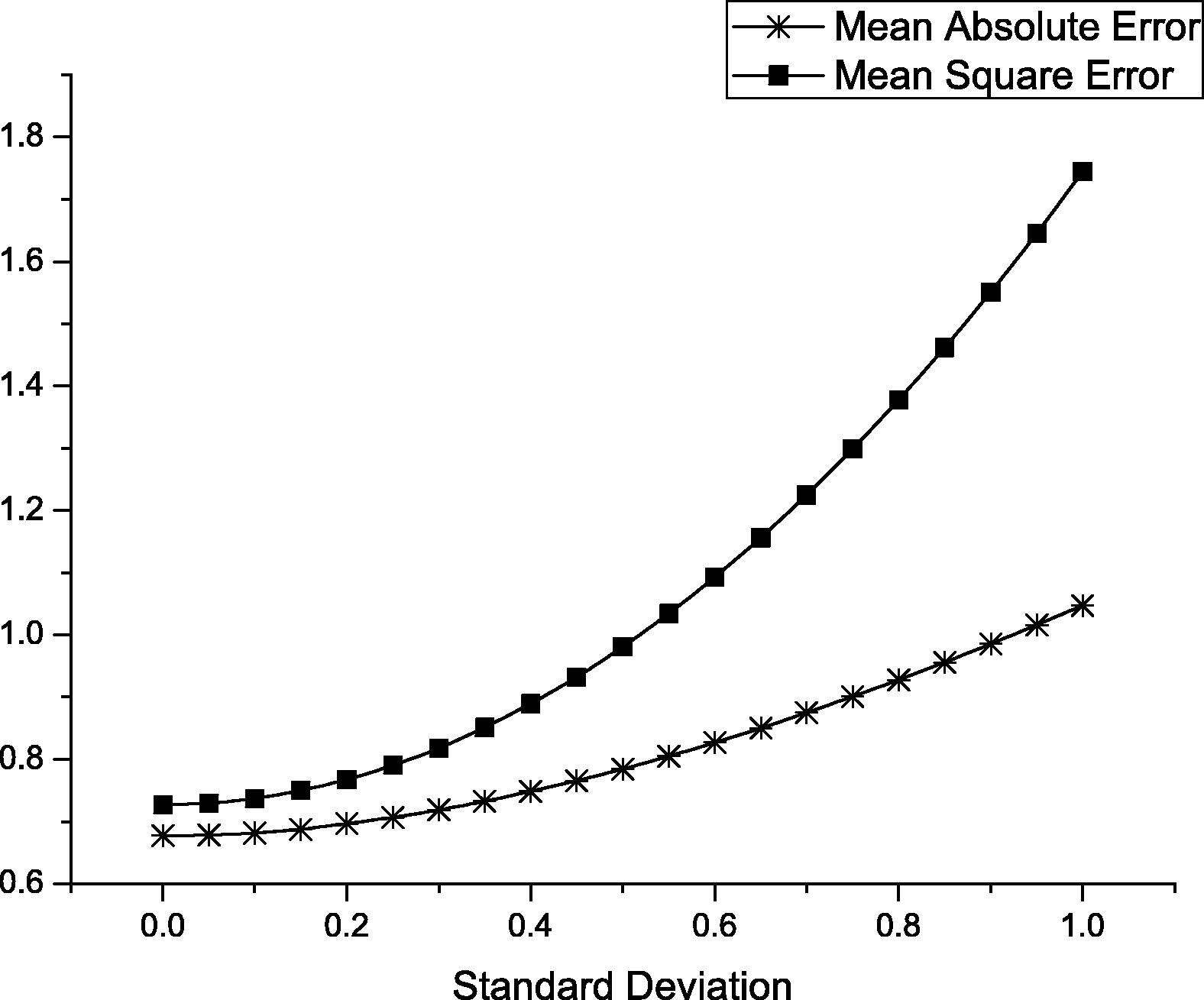
- Error estimation for normal distribution random predicator.
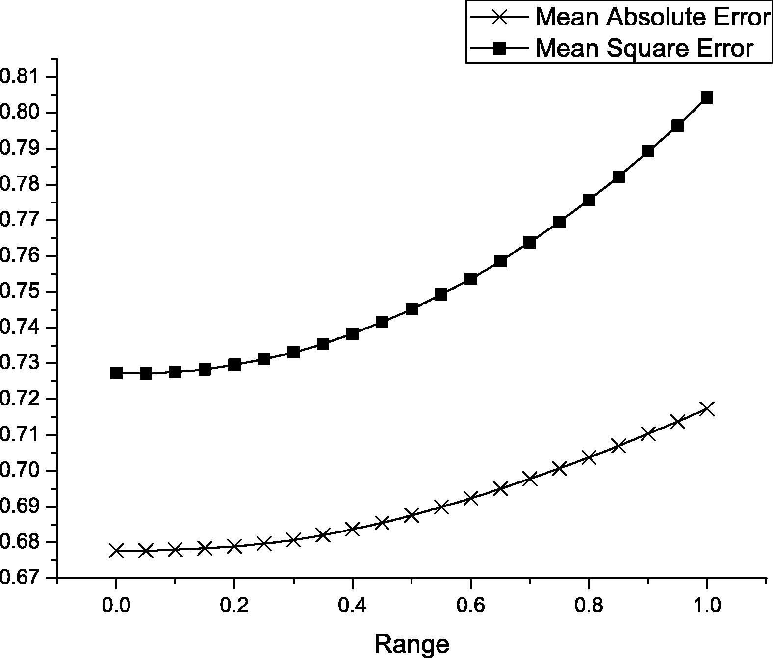
- Error estimation for uniform distribution random predicator.
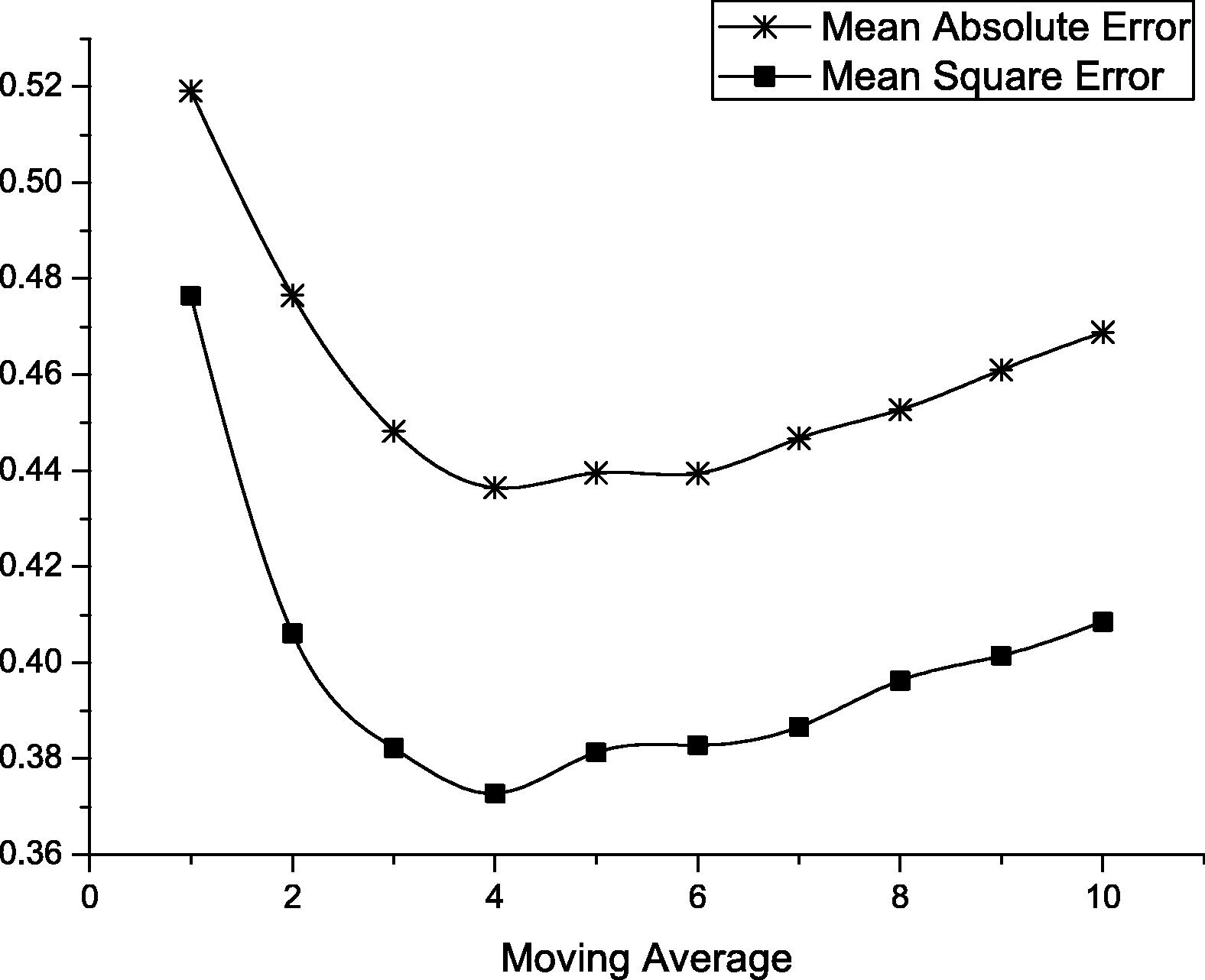
- Error estimation for moving average predicator.
| Prediction method | Accuracy metrics | |
|---|---|---|
| Average absolute error | Mean square error | |
| Moving average of 1 (previous magnitude occurs again) | 0.5191 | 0.4765 |
| Moving average of 2 | 0.4766 | 0.4062 |
| Moving average of 3 | 0.4482 | 0.3822 |
| Moving average of 4 | 0.4365 | 0.3728 |
| Moving average of 5 | 0.4396 | 0.3813 |
| Moving average of 6 | 0.4395 | 0.3828 |
| Moving average of 7 | 0.4467 | 0.3866 |
| Moving average of 8 | 0.4527 | 0.3963 |
| Linear y = −0.00019x + 3.9 | 0.6696 | 0.7309 |
| Quadratic y = 35 × 10−6 x2 + 12 × 10−3 x + 4.5 | 3.7906 | 19.5182 |
| Cubic y = −32 × 10−8 x3 + 19 × 10−5 x2 − 32 × 10−3 x + 5.1 | 0.6353 | 0.6167 |
| 4th degree y = −95 × 10−11 x4 + 29 × 10−8 x3 + 64 × 10−6 x2 − 22 × 10−3 x + 4.9 | 0.6270 | 0.6180 |
| 5th degree y = 69 × 10−12 x5 − 57 × 10−9 x4 + 16 × 10−6 x3 − 19 × 10−4 x2 + 67 × 10−3 x + 3.9 | 4.1772 | 36.7177 |
| 6th degree y = 13 × 10−14 x6 − 57 × 10−12 x5 − 11 × 10−9 x4 + 83 × 10−7 x3 − 12 × 10−4 x2 + 46 × 10−3 x + 4.1 | 0.9386 | 1.7128 |
6.2 Performance metrics
There are many performance metrics that can be used to evaluate and compare between forecasting methods such as time complexity, space complexity, and accuracy of the model. Although time – sometime space – is very important during training stage and may considered an obstacle, in this paper we focus on accuracy rather than time and space complexity because training stage is performed once. We have used two accuracy metrics to evaluate the performance over our model compared with other methods. These metrics are the following:
-
Mean absolute error (MAE): It is a quantity used to measure how close predictions are to the target outcomes. The mean absolute error is defined as following:
-
Mean squared error: It is a quantity used to measure the average of the square of the error from the target outcomes. The mean squared error is defined as following:
-
In MSE, the larger error will contribute more to the MSE value than small error. In other word, MSE penalizes larger errors and is generous toward small errors.
6.3 Performance results
In this section, we present the performance results for our neural network model compared to other forecasting methods. We have plotted the mean square error (MSE) and mean absolute error (MAE) for normally distributed random predictor as shown in Fig. 16, while Fig. 17 shows the mean square error (MSE) and mean absolute error (MAE) for uniformly distributed random predictor. We notice that, both methods start with the same performance since they represent the mean magnitude value at the beginning. However, normally distributed random predictor performs worse than uniformly distributed random predictor when the standard deviation value increase. These two figures illustrate clearly that earthquake magnitudes do not follow these statistical distributions which show how hard it is to predict magnitude using statistical tools. Furthermore, the two figures show that earthquake magnitude is not independent from pervious earthquake events so we cannot deal with earthquake events separately.
On the other hand, moving average performs much better than normally distributed random predictor and uniformly distributed random predictor as shown in Fig. 18. The figure shows the mean square error (MSE) and mean absolute error (MAE) for moving average method over different interval. The figure shows that moving average performs best when the interval value is four, so the last four earthquake magnitudes are enough to provide a best accuracy for moving average.
Other statistical fitting methods have been tested and their results are shown in Table 2. Similar to normally distributed random predictor and uniformly distributed random predictor, these statistical methods could not do better than moving average.
Finally, the performance of our neural network model is shown in Tables 3 and 4. Table 3 shows the accuracy for the top ten network configurations in terms of mean square error (MSE), while Table 4 shows the top ten network configurations in terms of mean absolute error (MAE). For the two tables, the second network configuration in Table 3 and the first one in Table 4 are the same. So that a network with the following configuration can be considered a better choice in terms of MSE and MAE together:
-
Delay = 3.
-
Number of neurons in the first hidden layer = 3.
-
Number of neurons in the second hidden layer = 2.
-
No third hidden layer.
-
The transfer function is Tansig.
| Network configuration | MSE | ||||
|---|---|---|---|---|---|
| Delay | Hidden Layer 1 | Hidden Layer 2 | Hidden Layer 3 | Transfer function | |
| 6 | 1 | 10 | × | Logsig | 0.114877 |
| 3 | 3 | 2 | × | Tansig | 0.115351 |
| 4 | 5 | 7 | × | Logsig | 0.122128 |
| 7 | 9 | 7 | 7 | Tansig | 0.122201 |
| 7 | 9 | 9 | 4 | Tansig | 0.127646 |
| 2 | 5 | 1 | × | Logsig | 0.12838 |
| 9 | 1 | 4 | 1 | Tansig | 0.128547 |
| 8 | 1 | 4 | 8 | Tansig | 0.129998 |
| 3 | 3 | 5 | 9 | Tansig | 0.13001 |
| 4 | 1 | 10 | × | Tansig | 0.131753 |
| Network configuration | MAE | ||||
|---|---|---|---|---|---|
| Delay | Hidden Layer 1 | Hidden Layer 2 | Hidden Layer 3 | Transfer function | |
| 3 | 3 | 2 | × | Tansig | 0.263717 |
| 7 | 9 | 7 | 7 | Tansig | 0.264596 |
| 8 | 6 | 3 | 2 | Tansig | 0.270434 |
| 6 | 1 | 10 | × | Logsig | 0.271525 |
| 8 | 1 | 4 | 8 | Tansig | 0.273067 |
| 7 | 9 | 9 | 4 | Tansig | 0.274606 |
| 5 | 4 | 10 | 2 | Tansig | 0.275836 |
| 8 | 3 | 3 | × | Tansig | 0.275973 |
| 10 | 8 | 3 | 6 | Tansig | 0.278503 |
| 9 | 1 | 2 | 6 | Tansig | 0.279328 |
For the results shown in this section, we notice that neural network has better capabilities to model data that has nonlinear and complex relationships between variables and can handle interactions between variables. Neural networks do not present an easily-understandable model. They are more of “black boxes” where there is no explanation of how the results were derived. The performance results show there is a great potential of using neural network for earthquake forecasting in northern Red Sear area, which needs to be investigated more.
7 Conclusions
Earthquake forecasting has become an emerging science, which has been applied in different areas of the world to monitor seismic activities and provide an early warning. Simple earthquake forecasting has been adapted in early ages using simple observations.
We presented a new artificial intelligent predication method based on artificial neural network to predict earthquake magnitude in the northern Red Sea region such as Gulf of Aqaba, Gulf of Suez and Sinai Peninsula . Other forecasting methods were used such as moving average, normal distributed random predictor, and uniformal distributed random predictor. In addition, we have presented different statistical methods and data fitting such as linear, quadratic, and cubic regression. We have presented a details performance analyses of the proposed methods for different evaluation metrics.
The results show that the neural network model provides higher forecast accuracy than other proposed methods. Neural network model is at least 32% better than other proposed methods. This is due to the fact that the neural network is capable to capture non-linear relationship than statistical methods and other proposed methods.
Acknowledgment
The Authors extend their appreciation to the Deanship of Scientific Research at King Saud University for funding the work through the research group project No RGP-VPP-122.
References
- A simple way to look at a Bayesian model for the statistics of earthquake prediction. Bulletin of the Seismological Society of America. 1981;71:1929-1931.
- [Google Scholar]
- PreSIS: a neural network-based approach to earthquake early warning for finite faults. Bulletin of the Seismological Society of America. 2008;98:366-382.
- [Google Scholar]
- Multi-layer neural network for precursor signal detection in electromagnetic wave observation applied to great earthquake prediction. IEEE-Eurasip Nonlinear Signal and Image Processing (NSIP) 2005 31–31
- [Google Scholar]
- Jusoh, M.H., Ya'acob, N., Saad, H., Sulaiman, A.A., Baba, N.H., Awang, R.A., Khan, Z.I., 2008. Earthquake prediction technique based on GPS dual frequency system in equatorial region. IEEE International RF and Microwave Conference, Springer, Berlin, pp. 372–376.
- Artificial neural network model for earthquake prediction with radon monitoring. Applied Radiation and Isotopes. 2009;67:212-219.
- [Google Scholar]
- Model dissection from earthquake time series: a comparative analysis using modern non-linear forecasting and artificial neural network approaches. Computers & Geosciences. 2009;35(2):191-204.
- [Google Scholar]
- Intermediate term earthquake prediction in the area of Greece: application of the algorithm M8. Pure and Applied Geophysics. 1990;134:261-282.
- [Google Scholar]
- On the correlation of seismicity with geophysical lineaments over the Indian subcontinent. Current Science. 2002;83:760-766.
- [Google Scholar]
- Layered neural networks based analysis of radon concentration and environmental parameters in earthquake prediction. Journal of Environmental Radioactivity. 2002;62(3):225.
- [Google Scholar]
- Experimental investigation of seismic damage identification using PCA-compressed frequency response functions and neural networks. Journal of Sound & Vibration. 2006;290:242-263.
- [Google Scholar]
- Self-organized maps based neural networks for detection of possible earthquake precursory electric field patterns. Advances in Engineering Software. 2006;37(4):207-217.
- [Google Scholar]
- Neural network models for earthquake magnitude prediction using multiple seismicity indicators. International Journal of Neural Systems. 2007;17:13-33.
- [Google Scholar]
- Recurrent neural network for approximate earthquake time and location prediction using multiple seismicity indicators. Computer-Aided Civil & Infrastructure Engineering (4):280-292.
- [Google Scholar]
- Estimation of focal parameters for Uttarkashi earthquake using peak ground horizontal accelerations. ISET Journal of Earthquake Technology. 1998;35:1-8.
- [Google Scholar]
- Plagianakos, V.P., Tzanaki, E., 2001. Chaotic analysis of seismic time series and short term forecasting using neural networks. In: Proceedings of the IJCNN ‘01 International Joint Conference on Neural Networks 3, Washington, DC, USA, pp. 1598–1602.
- Parallel distributed processing: explorations in the microstructure of cognition. Vol vol. 1. Cambridge: MIT; 1986. pp. 318−362
- Rundle, J., Tiampo, K., Klein, W., Martins, J., 2002. Self-organization in leaky threshold systems: The influence of near-mean field dynamics and its implications for earthquakes, neurobiology, and forecasting. In: Proceeding of National Academy of Sciences, USA, vol. 99, pp. 2514–2521.
- Shimizu, S., Sugisaki, K., Ohmori, H., 2008. Recursive sample-entropy method and its application for complexity observation of earth current. In: International Conference on Control, Automation and Systems (ICCAS), Seoul, South Korea, pp. 1250–1253.
- Su, You-Po, Zhu, Qing-Jie, 2009. Application of ANN to prediction of earthquake influence. In: Second International Conference on Information and Computing Science (ICIC’09), Manchester, vol. 2, pp. 234–237.
- Turmov, G.P., Korochentsev, V.I., Gorodetskaya, E.V., Mironenko, A.M., Kislitsin, D.V., Starodubtsev, O.A., 2000. Forecast of underwater earthquakes with a great degree of probability. In: Proceedings of the 2000 International Symposium on Underwater Technology, Tokyo, Japan, pp. 110–115.
- Physical properties of the variations of the electric field of the Earth preceding earthquakes I. Tectonophysics. 1984;110:73-98.
- [Google Scholar]
- Physical properties of the variations of the electric field of the Earth preceding earthquakes II. Tectonophysics. 1984;110:99-125.
- [Google Scholar]
- Official earthquake prediction procedure in Greece. Tectonophysics. 1988;152:193-196.
- [Google Scholar]
- Short-term earthquake prediction in Greece by seismic electric signals. In: Lighthill Sir J., ed. Critical Review of VAN: Earthquake Prediction from Seismic Electric Signals. Singapore: World Scientific Publishing Co.; 1996. p. :29-76.
- [Google Scholar]
- Estimation of the Earthquakes in Chinese Mainland by using artificial neural networks (in Chinese) Chinese Journal of Earthquakes. 2001;3(21):10-14.
- [Google Scholar]
- Predicting the 1975 Haicheng earthquake. Bulletin of the Seismological Society of America. 2006;96:757-795.
- [Google Scholar]
- Zhihuan, Zhong, Junjing, Yu, 1990. Prediction of earthquake damages and reliability analysis using fuzzy sets. In: First International Symposium on Uncertainty Modeling and Analysis, College Park, MD, USA, pp. 173–176.


